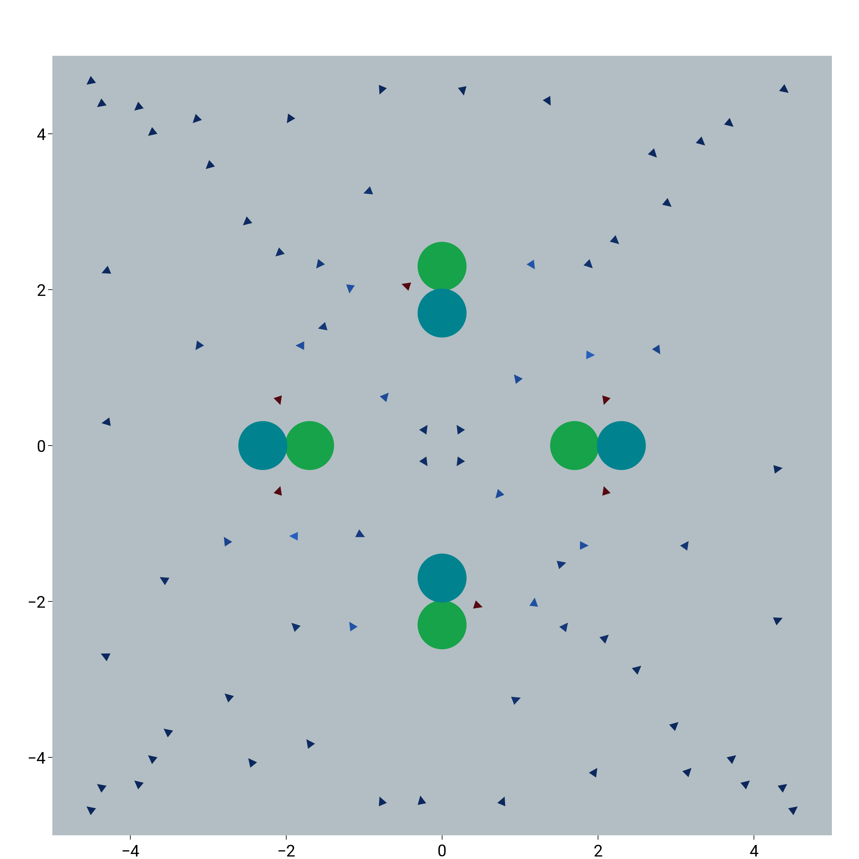
Magnetic Field Visualization

Four magnetic dipoles arranged on the cardinal axes generate the field plotted here. Three thousand short “iron filings” are oriented along the local field direction, then a streamplot superimposes smooth field lines coloured by magnitude with the dc.ice_fire colormap.

This example highlights:

• Mixing custom dm.mix_colors blends with built-in dartwork-mpl colormaps (dc.ice_fire).

• Marking dipole poles with red/blue Circle patches plus N/S labels for instant orientation.

/home/runner/work/dartwork-mpl/dartwork-mpl/docs/examples_source/08_creative_visualizations/plot_particles_magnetic_field.py:107: UserWarning: Setting the 'color' property will override the edgecolor or facecolor properties.
  Circle(
/home/runner/work/dartwork-mpl/dartwork-mpl/docs/examples_source/08_creative_visualizations/plot_particles_magnetic_field.py:127: UserWarning: Setting the 'color' property will override the edgecolor or facecolor properties.
  Circle(

import matplotlib.pyplot as plt
import numpy as np
from matplotlib.patches import Circle

import dartwork_mpl as dm

np.random.seed(42)
dm.style.use("scientific")

fig, ax = plt.subplots(figsize=dm.figsize("14cm", "square"))

dipoles = [
    {"pos": (-2, 0), "moment": (1, 0), "strength": 2},
    {"pos": (2, 0), "moment": (-1, 0), "strength": 2},
    {"pos": (0, 2), "moment": (0, 1), "strength": 1.5},
    {"pos": (0, -2), "moment": (0, -1), "strength": 1.5},
]


def magnetic_field(x, y, dipoles):
    Bx, By = 0, 0
    for dipole in dipoles:
        dx = x - dipole["pos"][0]
        dy = y - dipole["pos"][1]
        r = np.sqrt(dx**2 + dy**2) + 0.01
        mx, my = dipole["moment"]
        strength = dipole["strength"]
        dot = (mx * dx + my * dy) / r**2
        Bx += strength * (3 * dot * dx / r**2 - mx) / r**3
        By += strength * (3 * dot * dy / r**2 - my) / r**3
    return Bx, By


x = np.linspace(-5, 5, 40)
y = np.linspace(-5, 5, 40)
X, Y = np.meshgrid(x, y)

Bx = np.zeros_like(X)
By = np.zeros_like(Y)
for i in range(len(x)):
    for j in range(len(y)):
        Bx[j, i], By[j, i] = magnetic_field(X[j, i], Y[j, i], dipoles)

B_mag = np.clip(np.sqrt(Bx**2 + By**2), 0, 5)

n_filings = 3000
filings_x = np.random.uniform(-5, 5, n_filings)
filings_y = np.random.uniform(-5, 5, n_filings)

for i in range(n_filings):
    bx, by = magnetic_field(filings_x[i], filings_y[i], dipoles)
    b_mag = np.sqrt(bx**2 + by**2)

    if b_mag > 0.1:
        bx, by = bx / b_mag, by / b_mag
        color_intensity = min(1, b_mag / 3)
        color = dm.mix_colors("dc.ocean1", "dc.vivid3", alpha=color_intensity)
        length = 0.1
        ax.plot(
            [filings_x[i] - bx * length / 2, filings_x[i] + bx * length / 2],
            [filings_y[i] - by * length / 2, filings_y[i] + by * length / 2],
            color=color,
            lw=dm.lw(-1),
            alpha=0.4 + 0.4 * color_intensity,
        )

ax.streamplot(
    X,
    Y,
    Bx,
    By,
    color=B_mag,
    cmap="dc.ice_fire",
    linewidth=dm.lw(-1),
    density=0.8,
    arrowsize=1,
)

for dipole in dipoles:
    n_pos = (
        dipole["pos"][0] + dipole["moment"][0] * 0.3,
        dipole["pos"][1] + dipole["moment"][1] * 0.3,
    )
    s_pos = (
        dipole["pos"][0] - dipole["moment"][0] * 0.3,
        dipole["pos"][1] - dipole["moment"][1] * 0.3,
    )

    ax.add_patch(
        Circle(
            n_pos,
            0.3,
            color="dc.vivid2",
            edgecolor="white",
            linewidth=dm.lw(0),
            zorder=20,
        )
    )
    ax.text(
        *n_pos,
        "N",
        ha="center",
        va="center",
        fontsize=dm.fs(0),
        color="white",
        weight="bold",
    )

    ax.add_patch(
        Circle(
            s_pos,
            0.3,
            color="dc.ocean2",
            edgecolor="white",
            linewidth=dm.lw(0),
            zorder=20,
        )
    )
    ax.text(
        *s_pos,
        "S",
        ha="center",
        va="center",
        fontsize=dm.fs(0),
        color="white",
        weight="bold",
    )

ax.set_xlim(-5, 5)
ax.set_ylim(-5, 5)
ax.set_aspect("equal")
for s in ax.spines.values():
    s.set_visible(False)
ax.set_facecolor("dc.nordic0")

ax.text(
    0,
    5.5,
    "Magnetic Field Visualization",
    ha="center",
    fontsize=dm.fs(3),
    color="white",
    weight="bold",
)

dm.simple_layout(fig)
plt.show()