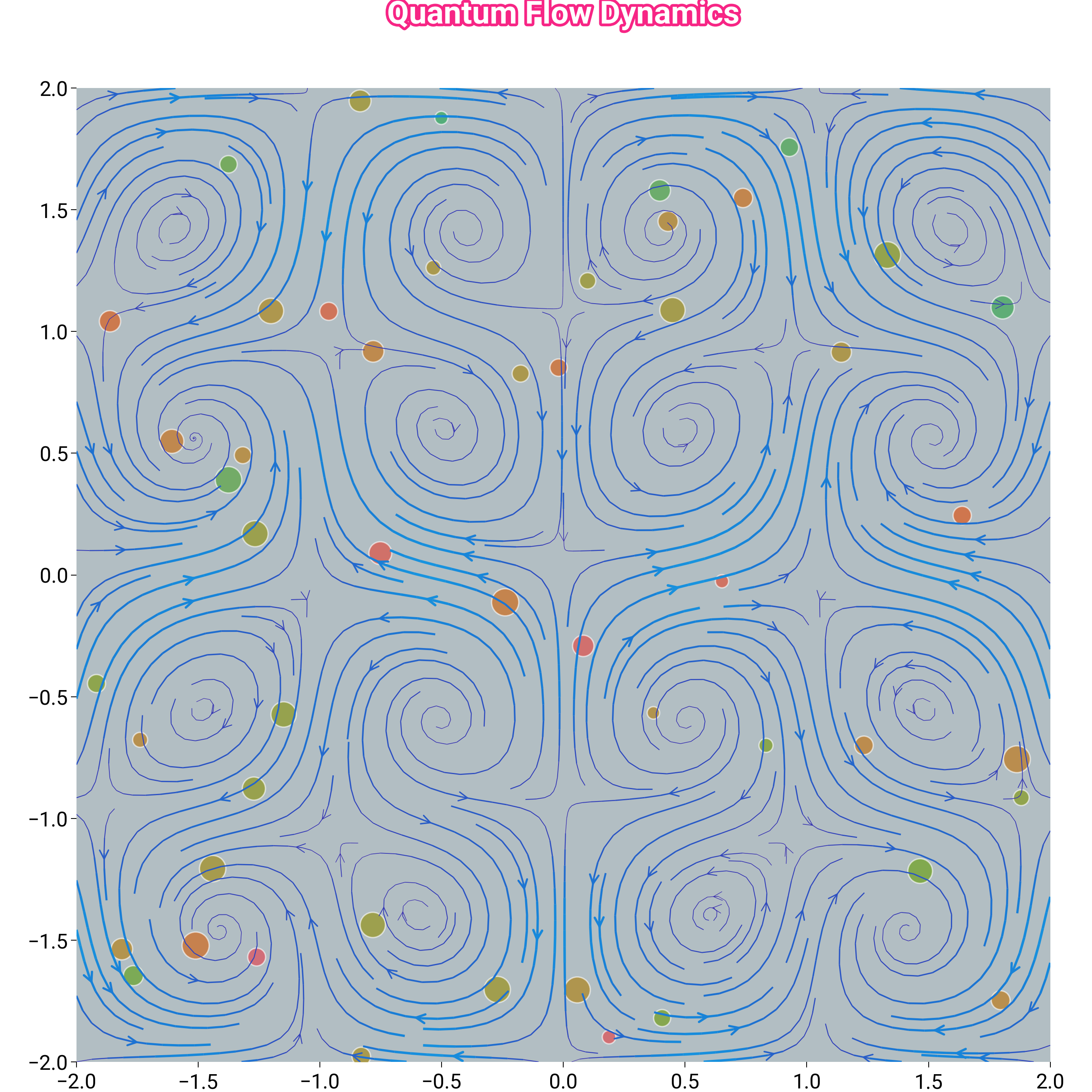
Quantum Flow Dynamics

A flow field with smooth OKLCH-interpolated streamlines, overlaid by a scatter of “particles” coloured along a pink-to-orange gradient. The streamline thickness is modulated by the local field magnitude, which gives the figure its turbulent, organic feel.

Highlights:

• dm.cspace(..., space="oklch") builds the colour ramp, then LinearSegmentedColormap.from_list wraps it as a Matplotlib cmap.

• path_effects.withStroke produces the glowing title.

import matplotlib.patheffects as path_effects
import matplotlib.pyplot as plt
import numpy as np
from matplotlib.colors import LinearSegmentedColormap

import dartwork_mpl as dm

np.random.seed(42)
dm.style.use("scientific")

fig, ax = plt.subplots(figsize=dm.figsize("14cm", "square"))

n_points = 25
x = np.linspace(-2, 2, n_points)
y = np.linspace(-2, 2, n_points)
X, Y = np.meshgrid(x, y)

t = 2.5
U = np.sin(np.pi * X) * np.cos(np.pi * Y) + 0.3 * np.sin(t * X)
V = -np.cos(np.pi * X) * np.sin(np.pi * Y) + 0.3 * np.cos(t * Y)
M = np.sqrt(U**2 + V**2)

colors_flow = dm.cspace("dc.cyber5", "dc.ocean1", n=256, space="oklch")
flow_cmap = LinearSegmentedColormap.from_list(
    "flow", [c.to_hex() for c in colors_flow]
)

ax.streamplot(
    X,
    Y,
    U,
    V,
    color=M,
    cmap=flow_cmap,
    linewidth=dm.lw(0) * M / M.max(),
    density=2,
    arrowsize=0.8,
    arrowstyle="->",
)

n_particles = 50
px = np.random.uniform(-2, 2, n_particles)
py = np.random.uniform(-2, 2, n_particles)
particle_colors = dm.cspace("dc.vivid2", "dc.sunset2", n=n_particles)

for x_p, y_p, color in zip(px, py, particle_colors, strict=False):
    size = np.random.uniform(20, 100)
    ax.scatter(
        x_p,
        y_p,
        s=size,
        c=[color.to_hex()],
        alpha=0.6,
        edgecolors="white",
        linewidths=0.5,
    )

for s in ax.spines.values():
    s.set_visible(False)
ax.set_xlim(-2, 2)
ax.set_ylim(-2, 2)
ax.set_aspect("equal")
ax.set_facecolor("dc.nordic0")

title = ax.text(
    0,
    2.3,
    "Quantum Flow Dynamics",
    ha="center",
    va="center",
    fontsize=dm.fs(4),
    fontweight=dm.fw(3),
    color="white",
)
title.set_path_effects(
    [path_effects.withStroke(linewidth=dm.lw(1), foreground="dc.cyber2")]
)

dm.simple_layout(fig)
plt.show()