Design rationale

This page explains why the design system’s colors — and eventually its typography — are built and gated this way. It separates design choices, implementation contracts, measured catalog evidence, and limits so readers can judge each claim at the right scope.

Modeled relative CIE Y (relative_y) is calculated from nominal D65 sRGB; it is not a measurement of a particular display, perceived brightness, or OKLab L.

To use the color surfaces directly, see Colors, Palettes, Colormaps, and Color class. Every figure below is rendered live from the shipped package by docs/color_system/generate_theory_figures.py, so the pictures are reproducible evidence for the named build.

Note

How to read the evidence

• Design choice names an intended property or accepted trade-off.

• Implementation names behavior pinned by the shipped software contract.

• Evidence reports a result for the stated data, model, and protocol.

• Limits state what that result does not measure or guarantee.

Tip

The decision in plain language

OKLab is a perceptually oriented working model, and OKLCH is its cylindrical coordinate view. The model gives the compiler useful lightness and distance coordinates; it is not a perfectly uniform law of vision.

The shipped catalog also retains its modeled relative-Y targets where the compatibility contract requires them. A new, intentionally incompatible color system could use direct OKLCH L and choose different output rules. The extra Y lock is a compatibility promise, not a law of color theory.

CIELAB, CIEDE2000, and named color-vision simulations do not construct the colors. They are model-specific checks on finished output. WCAG contrast answers a pairwise question for a named foreground and background.

Note

Four rulers, four different jobs

• OKLab and OKLCH are two coordinate views of the same perceptually oriented working model. OKLab L, a, and b are Cartesian coordinates; OKLCH expresses the same point with L, chroma C, and hue h.

• ΔEOK×100 is 100 times the raw Euclidean distance in Oklab. Multiplying by 100 changes displayed units, not ranking, equalized positions, or CV.

• On the normalized modeled-relative-Y scale defined above, 0 means nominal black and 1 means nominal reference white. This is modeled relative CIE Y calculated from nominal D65 sRGB, not an observer or device measurement.

• Catalog relative_y and WCAG relative luminance are closely related decoded-sRGB Y-like calculations with separately pinned coefficient conventions. WCAG adds a pairwise contrast ratio for a specified foreground/background pair.

CIELAB, CIEDE2000, and the named color-vision-deficiency (CVD) simulations are model-specific finished-output checks. Protan and deutan are red-green deficiency classes; tritan is a blue-yellow deficiency class. Each result is a model-specific regression diagnostic, not a construction coordinate, observer guarantee, or accessibility certification. A simulation result is not a guarantee for every individual observer.

Four principles

1 · One construction model. Color construction uses OKLab L in the perceptually oriented OKLab model and authors chroma and hue through its cylindrical OKLCH coordinate view. Where a topology specifies path-distance placement, spacing uses ΔEOK×100; other topologies retain their explicit placement rules. CIELAB and CIEDE2000 do not drive the recipe or compiler.

2 · Generative, not tabular. Colors are not authored as hand-picked tables; they are computed and stored as generated outputs. Each family is defined by a handful of numbers, and a compiler turns those numbers into a 10-step ladder.

Consistency is enforced because every family passes the same rules. Extension is principled because a new hue axis is a point on a curve, not a guess. The design is verifiable because the per-family values lie on smooth low-order curves rather than being unrelated choices.

3 · Separate compatibility output from perception. The retained catalog contract is modeled relative_y, not a second perceptual lightness model. A recipe tone means neutral_tone = cbrt(relative_y). For the shipped catalog, the relative-Y solver searches chromatic OKLCH L at the requested C and h; the common gamut mapper may then reduce C while preserving the resulting L and h.

4 · Honest validation. The validation-only layer retains CIELAB, ΔE00, and named CVD simulations as model-specific regression diagnostics on finished colors. They do not control construction or certify accessibility.

WCAG relative luminance uses a separately pinned coefficient convention, then adds a ratio for a specified foreground/background pair. No single metric makes a palette perfectly uniform.

The construction foundation (axiom A1)

A1 — author color coordinates in OKLab/OKLCH, apply ΔEOK×100 arc-length placement only to the recipe paths that specify it, and retain catalog relative_y as an explicit compatibility contract. For requests whose OKLCH L is in range and chroma is non-negligible, pre-quantization gamut mapping holds L and h constant while reducing C. CIELAB/ΔE00/CVD remain model-specific finished-output diagnostics, and WCAG contrast remains a pairwise check.

The chromatic single-hue, continuous gray, and multi-hue sequential paths use ΔEOK arc-length resampling. The 11 diverging maps use pointwise symmetric arm construction followed by integer-index resampling; hue samples equal hue angles; and halo and corona use closed-path ΔEOK arc-length resampling. Discrete gray is the additional exception described in A6. These distinctions are part of construction, not validation.

Note

Gamut mapping in plain language

sRGB cannot display every OKLCH request. When a requested color is outside that displayable range, the mapper applies a narrow coordinate contract. For requests whose OKLCH L is in range and chroma is non-negligible, the pre-quantization bisection holds L and h constant while reducing C. Bisection repeatedly halves the remaining search range; the boundary search stops at the implementation’s numeric tolerance. Near neutral, hue is powerless as a coordinate and numerically unstable, so no hue-preservation claim applies there. The final residual channel clamp and 8-bit serialization can perturb reconstructed OKLCH coordinates. Out-of-range achromatic lightness maps to black or white. This is a coordinate-preserving boundary policy, not a perceptual minimum-difference or global appearance optimization, and it does not preserve appearance exactly.

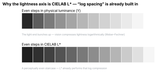
neutral_tone is the recipe’s output coordinate: relative_y = tone³. Actual chromatic OKLab L is a result coordinate and can differ at the same tone because hue and chroma affect modeled relative Y. Keeping these names separate prevents a tone target from being mistaken for perceptual lightness.

Note

What these statistics mean

The coefficient of variation (CV) compares the spread of neighboring distances with their mean. Lower CV means more even neighboring distances for the named sample; it does not prove that every observer sees perfectly equal steps. R² = 1 means a perfect fit to the specified model, so a value closer to 1 is a better fit to that model, not proof that the model is universal. wRMSE is weighted fit error, so lower is better; it summarizes the named weighted data and is not itself a perception guarantee.

Why OKLab/OKLCH throughout construction. OKLab supplies the canonical L, a, b coordinates and ΔEOK path distance. Its cylindrical OKLCH view makes C and h convenient to author. A bounded ΔEOK coefficient of variation makes the ten steps more consistent; it does not assert that equal numbers guarantee exactly equal visual differences for every observer.

Note

Map words used below

For forward/default registrations:

• Single-hue sequential: low values are light and high values are dark.

• Multi-hue sequential: low values are dark and high values are light.

• Diverging: two poles around a light center; no one monotonic low-to-high direction applies.

• Cyclic: no low/high direction; the generating path closes, as with angles returning from 360° to 0°.

• Qualitative: unordered categories rather than numeric values.

• _r swaps the endpoint assignment for a registered continuous map.

• The seam is the join between a cyclic map’s end and start.

• Isoluminant means designed to keep relative_y constant while hue changes; it does not promise equal perceived brightness.

Maintainers call a map’s required output shape its topology: an ordered path, two matched arms, or a closed loop. A topology gate simply rejects output that breaks that required shape.

Note

What LUT means

A lookup table (LUT) is the ordered 256 colors shipped behind one continuous map. A renderer samples that stored sequence when it converts numeric values to colors. For a cyclic map, the continuous generating path includes a closing endpoint, but the shipped 256-entry LUT is endpoint-exclusive. Its first and last stored entries differ by one ordinary wrap step; they are not duplicate endpoints.

Why retain a relative-Y lock. relative_y preserves the published nominal source-color ordering and continuous-map topology without asking CIELAB to drive construction. It is a compatibility requirement, much like a pinned numeric output budget. The unlocked diagnostic uses the same recipe and pre-limited chroma, rendered with L=tone; it isolates the relative-Y-lock effect and does not compute a new direct-L maximum-chroma boundary.

This lock is not a universal law of color theory. A new, intentionally incompatible system could define L=tone and adopt different output rules. dartwork-mpl keeps the lock because the published palette and 43×256 LUTs, their modeled-relative-Y topology and behavior are compatibility contracts. Simply reinterpreting the migrated tone values as direct OKLCH L changes those outputs and breaks ordered/symmetric-map gates. The extra solve is therefore justified by an explicit compatibility promise, not by a need to mix CIELAB into construction.

Gamut mapping. When an OKLCH request falls outside sRGB, channel clipping can skew hue. For an in-range L and non-negligible chroma, the named pre-quantization bisection holds the requested OKLCH L and h and reduces C until the color is in gamut. Near neutral, hue has no effective leverage; outside the achromatic lightness interval, the result is black or white. Final clamping and 8-bit serialization can slightly perturb reconstructed coordinates. No CIELAB target participates in this mapping.

The generation design rules (A2–A8)

These are bounded catalog rules, not laws of color perception. Each rule names its design intent, current implementation, local evidence or illustration, and limits so that a catalog choice is not mistaken for a universal claim.

Tip

How to read A2–A8

Each design rule answers one practical question:

• A2: How dark may each hue family go while retaining its identity?

• A3: How colorful should each hue become, and where should it peak?

• A4: How should hue turn as a family gets darker?

• A5: Where should the ten named steps sit along the path?

• A6: What changes for gray, which has no chromatic identity?

• A7: What must pass before an output can be released?

• A8: Why are colormap ranges chosen per topology and scene?

A2 · hue-specific dark endpoints

Every family follows a shared top tone and descends to a hue-specific tone_floor. The floor is not the gamut wall: it is a design value defined by a Fourier curve over hue and interpreted through relative_y = tone³.

Design intent. Each family stops where the shipped catalog keeps the dark character chosen for that family. This is catalog art direction, not a psychophysical law. During catalog review, forcing the authored endpoints to one modeled-relative-Y minimum made the warm families look muddy. That is design history and judgment, not measured evidence.

Implementation. The accepted model puts tone_floor(h) on a Fourier (k=3) curve. The v6 tone values were migrated once from the accepted v5 output targets and are now stored directly; production does not convert CIELAB values at runtime. A new family’s floor is read from the tone curve.

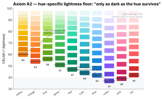
Evidence. In the accepted catalog, yellow has a higher tone floor than violet.

Limits. tone_floor records the accepted catalog endpoint. It is neither the sRGB gamut boundary nor an experimentally measured threshold at which a hue stops being identifiable for every observer.

A3 · chroma — hue fingerprint × shared shape

Peak chroma C_max(h) is a smooth function of hue (Fourier k=3); the chroma ladder uses one shared rise-peak-fall functional form and shared exponents. C_max, t_p, c_0, and c_end vary by family.

Design intent. The families use one chroma grammar while retaining different scales, peak locations, and endpoint ratios. A3 shares a functional form, not every parameter.

Implementation. Every family uses the same rise-peak-fall functional form and shape exponents. The scale (C_max), peak position (t_p), pastel-start ratio (c_0), and dark-end ratio (c_end) are family parameters. For example, red peaks dark (t_p=0.85) while yellow peaks mid-ladder (t_p=0.45).

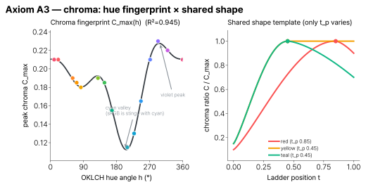
Evidence. Evaluating the Fourier curve at each family’s mid-hue gives an in-sample R² of 0.997 across the authored nineteen-family catalog.

Limits. The fit describes those authored C_max values. It is not predictive validation, proof of the sRGB gamut boundary, or a claim that the family peak positions are quality scores.

A4 · catalog hue drift

Hue rotates along path progress: h(t) = h₀ + Δh · t^γ. As the path moves toward its dark tone endpoint, warm hues rotate a lot (toward flame-like orange/red), cool hues a little.

Design intent. The accepted warm families turn toward orange/red at their dark ends, while the cool families turn less. This warm-hue drift is catalog art direction, not a psychophysical law.

Implementation. Every chromatic family uses h(t) = h₀ + Δh · t^γ. The per-family Δh selects the endpoint rotation, and γ selects when that rotation occurs; γ>1 concentrates it toward the dark end.

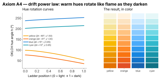
Evidence. Yellow rotates Δh −46° (bright lemon → dark amber), while blue rotates +15°. One power law fits the authored family paths to wRMSE ≤ 1.7°.

Limits. The weighted fit error supports one compact description of this catalog. It does not establish identical perceived hue motion, preferred dark endpoints, or equal vividness for every observer.

A5 · chromatic ΔEOK arc-length step placement

Each 10-step chromatic family ladder is placed at equal arc-length intervals along its rendered path under ΔEOK. The gray exception is specified in A6.

Design intent. Fixed path-distance placement makes a two-index move a useful approximation to the same amount of travel elsewhere in one family.

Implementation. For chromatic family ladders, the only shipped placement policy is fixed ΔEOK arc-length equalization. There is no public ease, exp, log, or spacing-warp option.

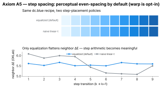
Evidence. Equalized spacing flattens the neighbor ΔEOK profile relative to naive linear-t sampling. That makes index differences a useful approximation (blue3↔blue5 and blue6↔blue8 cover similar path lengths).

Limits. ΔEOK equalization is model-specific and is not an exact law of perception. Alternative placement policies are possible only as future, incompatible designs; shipping one would require an explicit public API and a compatibility contract.

A6 · the near-neutral gray exception

Design intent. Gray is near-neutral, with a deliberate cool tint, so it can serve grids, reference lines, benchmarks, and “other” categories without competing with the chromatic families.

Implementation. The gray ladder directly samples ten evenly spaced neutral-tone positions on the shared modeled-Y path at h250, using the stored chroma profile with C ≤ 0.011. It does not call the chromatic-family equalizer. Its resulting neighbor ΔEOK near-evenness is measured and protected by frozen non-regression gates. The separate continuous-gray colormap does use continuous ΔEOK arc-length resampling. The shipped ladder retains that small nonzero chroma. Gray is not part of Octave (dc.octave); Octave Print adds a dark gray as its eighth color for a distinct historical neutral-coordinate diagnostic.

Evidence. No user-study or task-performance protocol has established that the cool tint improves those chart roles. A6 records a design choice rather than a measured benefit.

Limits. The word “gray” names the catalog role. The colors are not perfectly achromatic, and the cool tint is not a guarantee of perceptual neutrality for every observer or surround.

A7 · per-asset release gates

Design intent. Release validation preserves exact public output and rejects metric regressions relative to the accepted asset, rather than turning one design-time threshold into a universal color rule.

Implementation. Current quality gates are per-asset frozen-baseline non-regression checks on raw, unrounded values. Exact mismatches or a listed quality regression fail the color-authority comparison.

Release surface	Current contract	Raw metric or authority
Exact public surfaces	names, order, colors, and discrete selections reproduce the published catalog with zero mismatches	strict frozen compatibility payload
Every direct-32 and full-256 row	count and degenerate-neighbor status match; step CV does not exceed its asset baseline	count, zero-step presence, and ΔEOK×100 step CV
Ordered palette and sequential/multi-hue direct-32/full-256 rows	preserve direction, modeled-relative-Y/OKLab-L monotonic floors, and modeled-relative-Y span; ordered direct-32 step CV ≤ min(v5, 0.08)	direction, oriented neighbor minima, span, and step CV
Ordered sequential/multi-hue full-256 rows	the weakest adjacent normal-sRGB pair has non-negative modeled-relative-Y margin after expanding both stored colors to their local half-step 8-bit round-to-even cells	oriented_delta_y + local_tolerance >= 0 at the recorded worst pair
Diverging/cyclic direct-32 and every quantized full-256 row	step CV does not regress from that asset’s frozen v5 value	per-asset ΔEOK×100 step CV
Categorical rows	normal, protan, deutan, tritan, and common minimum separations do not regress	per-asset CIEDE2000 minima after the named CVD pipelines
Diverging full-LUT topology	center, both arms, arc/step balance, and mirrored modeled-relative-Y/ΔEOK summaries do not regress	per-asset diverging topology record
Cyclic full-LUT topology	topology kind and seam metrics do not regress; hue retains its isoluminant modeled-relative-Y spread, while twilight maps retain their two-arm records	per-asset seam ΔEOK/CIEDE2000, modeled-relative-Y, and arm/mirror records

The categorical pipeline starts from catalog hex colors, decodes nominal sRGB to linear sRGB, applies the named full-severity Machado (2009) protan/deutan or Brettel–Viénot–Mollon (1997) tritan simulation, clamps simulated channels and re-encodes nominal sRGB, applies the catalog’s 8-bit hex quantization convention, converts the quantized results to CIELAB, and compares every pair with CIEDE2000.

Evidence. The frozen oracle is checked with published Sharma et al. CIEDE2000 reference pairs, source-pinned Machado (2009) matrices, project-adapted Brettel–Viénot–Mollon (1997) matrices, and project-derived CVD regression cases before candidate metrics are compared. The common-CVD 10 and tritan 8 thresholds were historical Octave search criteria; they selected the accepted rows but are not universal categorical minima or the current shared release policy.

The full-256 quantization margin is an encoding proof, not a perceptual threshold. It asks only whether the intended normal-sRGB modeled-Y order is possible inside the two local 8-bit cells. CVD results keep model-specific per-asset regression checks instead of borrowing that normal-sRGB proof.

Limits. These gates show non-regression under named software models and accepted baselines. CVD simulation does not represent every observer, and a passing row is not a general accessibility certification.

WCAG remains outside the color-authority compile-gate table. A tested pairwise contrast ratio and threshold is a separate check for a specified foreground/background pair; it does not certify the catalog.

A8 · palette-floor-independent, topology-specific ranges

Continuous-map ranges are palette-floor-independent but class- and scene-specific. They do not inherit each palette family’s hue-specific tone_floor.

Design intent. Each continuous map needs enough output range for its own ordered, diverging, or cyclic scene without forcing every topology through one range contract.

Implementation. Single-hue ramps, multi-hue sequential scenes, diverging pairs, and cyclic maps use their own class- and scene-specific endpoint and topology recipes instead of palette family floors.

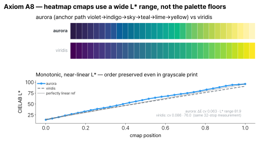
Illustration. This is a bounded same-protocol benchmark under the displayed 32-stop sampling: aurora reports ΔEOK cv 0.063, actual-OKLab-L span 0.696, and modeled-relative-Y span 0.884; viridis reports 0.086, 0.633, and 0.763 respectively. Lower CV is more even, so these measurements show a lower step-variation coefficient for aurora in this sample. A larger span means more range on the named coordinate, so aurora also covers wider actual-OKLab-L and modeled-relative-Y spans here. The comparison does not establish perfect perceptual uniformity or universal perceived-brightness range.

Limits. Cross-panel comparison of the same variable requires the same colormap, direction, and normalization, including identical limits or the same Normalize object. Different maps are not one comparable color scale. Even then, the reported spans and CV describe the named coordinates and sampling protocol rather than universal perception.

Anatomy of a family

The generated dc.* ramps are not hand-picked tables of hex codes. Their palette-authoring recipe uses the bookkeeping and scalar-leaf counts below. Continuous maps carry additional topology-specific recipe data, while curated categorical sets are a separate, preserved manual surface. These figures describe palette authoring, not the MCP API (which exposes 16 tools, 10 resources, 4 resource templates, and 2 prompts).

The generated system has two related recipe counts. Its bookkeeping total is 107 named slots:

• 19 chromatic families × four free authoring fields = 76 named slots;

• four third-order Fourier series × six coefficients = 24 named slots; and

• seven named constants = seven slots.

GRAY_C_PROFILE contains ten numbers but counts as one named constant. With the same exclusions, this corresponds to 116 scalar numeric leaves. TONE_DERIVATION_GRID is migration-only and excluded from both totals.

Shipped family records store all eight operational values. The four authored fields are h₀ (hue anchor), Δh (total drift), γ (drift timing), and t_p (chroma-peak position). The four Fourier-derived fields are C_max, tone_floor, c₀, and c_end; they are an extension prior/mechanism, not recomputed for every current row at runtime.

Gray makes the single-hue catalog 20 families total but follows its shared achromatic constants instead of a chromatic family row. The hand-tuned curated sets are preserved outputs, not part of either recipe count. Continuous maps carry additional topology-specific recipes, so 107 is not the input count for the entire continuous catalog.

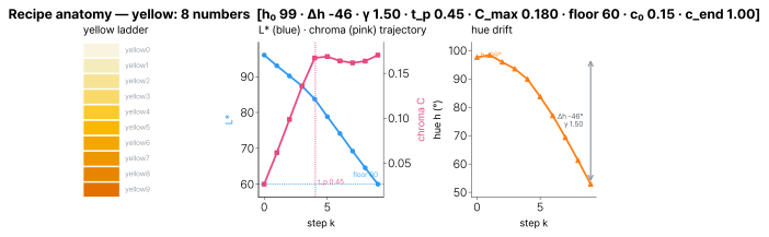
The yellow inputs and derived values drive four distinct traces: recipe tone, rendered catalog relative_y, actual OKLab L, and the OKLCH C/h path. The separation is deliberate: tone is not another spelling of chromatic L.

The historical parameter grid below is retained to explain the exact v5→v6 migration. The legacy floor L* column is provenance only: v6 stores the derived 0–1 tone_floor and production performs no CIELAB conversion. Other values are rounded for readability and are not a replacement SSOT.

family	h₀	Δh	γ	t_p	C_max	legacy floor L*	c₀	c_end
red	16	+11	1.10	0.85	0.210	42	0.10	0.90
rose	3	+14	1.00	0.85	0.210	40	0.10	0.85
coral	27	+2	1.15	0.85	0.205	44	0.10	0.90
tangerine	52	−12	1.20	0.85	0.195	49	0.15	0.95
orange	77	−41	1.30	0.85	0.190	54	0.15	1.00
amber	88	−44	1.40	0.65	0.185	57	0.15	1.00
yellow	99	−46	1.50	0.45	0.180	60	0.15	1.00
lime	122	+11	0.60	0.45	0.190	56	0.15	0.85
green	149	−3	0.60	0.50	0.185	51	0.15	0.75
teal	176	−13	0.60	0.45	0.155	47	0.15	0.70
cyan	202	+13	0.85	0.45	0.115	44	0.15	0.75
sky	220	+14	0.85	0.60	0.130	43	0.15	0.80
blue	238	+15	0.85	0.75	0.165	42	0.15	0.85
cobalt	256	+5	1.25	0.80	0.190	40	0.15	0.85
indigo	273	−5	1.65	0.85	0.210	39	0.10	0.85
violet	298	−12	1.25	0.85	0.230	37	0.10	0.85
purple	319	+0	1.00	0.75	0.220	37	0.05	0.85
fuchsia	335	+9	0.95	0.80	0.210	37	0.05	0.85
pink	350	+18	0.85	0.85	0.210	39	0.05	0.85

gray follows the A6 neutral-tone rule with a cool tint at h250. Its historical v5 endpoints were L* 96→28; those numbers are migration provenance, not live recipe inputs. A new chromatic family needs only its four free numbers — the rest is read from the global curves.

The metric system — what the ruler is

A color system’s credibility depends on which ruler owns which decision. The current system separates four roles without pretending that each name denotes an unrelated physical quantity:

Purpose	Coordinate or metric	Role
Construction	OKLab L, OKLCH C/h, ΔEOK×100	authoring and topology-specific path placement in one perceptually oriented model
Catalog compatibility	relative_y from nominal D65 sRGB	accepted ordering, symmetry, and the hue isoluminant contract
Finished-output diagnostics	CIELAB, CIEDE2000, Machado/BVM CVD	model-specific regression diagnostics only
Text contrast	WCAG relative luminance plus contrast ratio	pairwise result for a specified foreground/background pair

Catalog relative_y and WCAG relative luminance both decode sRGB and form a Y-like weighted sum. Their separately pinned coefficient conventions are a software-compatibility detail, not evidence of two unrelated phenomena. WCAG then adds its pairwise contrast-ratio formula.

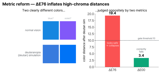
This is an important regression-model correction inherited from v5. An earlier diagnostic used ΔE76 (CIELAB Euclidean), which assigns a larger distance to this high-chroma pair under the named simulation.

blue7 and violet7 are distinct in their unsimulated nominal-sRGB rendering but nearly merge under the named deutan simulation. ΔE76 puts the pair above the historical regression threshold, while CIEDE2000 puts it below that threshold.

That result motivated switching the shipped regression diagnostic to CIEDE2000 and re-searching the cycle. It does not establish that either score is an observer guarantee or accessibility certification.

The diagnostics publish multiple model-specific rulers. Equalizing ΔEOK steps does not simultaneously equalize CIEDE2000 distances, modeled-relative-Y increments, or separations after a named CVD simulation. Being explicit about what is constructed and what is only validated is the honest design (principle 4).

The CVD validation model is chosen per deficiency. The common red-green deficiencies (protanopia and deuteranopia) use Machado et al. (2009) at full severity. Tritanopia uses the Brettel–Viénot–Mollon (BVM, 1997) projection.

The common-CVD 10 and tritan 8 floors were historical Octave selection criteria, not current shared release gates. Under the named full-severity simulation diagnostics, dc.octave measures 10.3 (common) / 8.3 (tritan) for Octave; dc.octave_print, 10.4 / 9.8 for Octave Print. For these simulated minimum distances, higher is better because it means the nearest pair remains farther apart. The scores apply only to the named models and severity, not every observer or viewing condition, and they do not certify accessibility.

Octave Print is hue-parallel with Octave — same hue per slot, with the violet slot matching and the dark gray anchor in slot eight. Its historical CIELAB neutral-coordinate diagnostic records a minimum pairwise ΔL* of 7.7. A larger minimum means more source-color separation under that bounded calculation; it does not model a particular printer, paper, conversion workflow, background, overlap, or observer, and does not by itself guarantee readable text. These validation numbers do not feed color selection in the v6 compiler.

Colormaps, derived from the palette

The continuous colormaps use the same OKLab/OKLCH construction and modeled relative-Y compatibility policy as the palette: 43 continuous maps across four kinds.

A separate set of 13 qualitative colormaps comprises the two Octave cycles and 11 curated qualitative sets. dm.list_colors() therefore returns 56 family records. The qualitative rows are registrations, not extra continuous recipes.

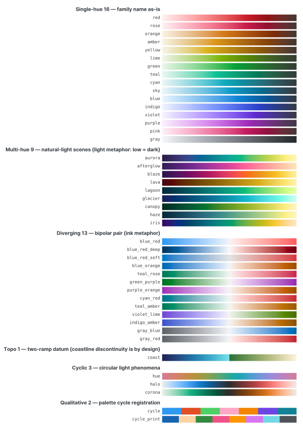
The continuous catalog: 20 single-hue ramps, 9 multi-hue scenes, 11 diverging pairs, and 3 cyclic maps. Qualitative registrations are cataloged separately.

One naming grammar. The name states color identity; the suffix states a variant.

Kind	Rule	Example
color token	dc.{family}{step}	dc.blue6
categorical cycle	octave · octave_print	dm.set_colors()
single-hue cmap	the family name itself	cmap="dc.blue"
multi-hue cmap	a natural-light scene name	dc.aurora
diverging cmap	a low_high pair name	dc.blue_red
cyclic cmap	a circular-light-phenomenon name	dc.halo
qualitative cmap	stable public cycle token	dc.octave
continuous-map variant suffix	_r (reverse)	dc.aurora_r

Direction — an ink/light metaphor. The metaphor applies to the two sequential classes, not every topology. For forward/default registrations, single-hue sequential maps assign low values to light colors and high values to dark colors; multi-hue sequential maps assign low values to dark colors and high values to light colors. Diverging maps have two poles around a light center, cyclic maps have no low/high direction, and qualitative maps are unordered.

This replaces matplotlib’s unprincipled mix of directions (Blues runs light→dark, viridis runs dark→light) with explicit sequential rules. _r is registered only for continuous maps and swaps the endpoint assignment. Reverse qualitative palettes with dm.colors(..., reverse=True).

Anchor-graph coherence. The 19 chromatic h₀ anchors describe palette identity and multi-hue scene waypoints; they are not the only hue source. A single-hue map renders one family identity, and a multi-hue map interpolates through the named waypoints. Diverging recipes may use rendered poles, and cyclic recipes may traverse a full hue circle. Their generating paths still share the catalog’s construction and validation contracts.

Palette, cycle, and colormap all live on one graph.

The multi-hue scenes

Multi-hue maps traverse several hues while retaining an ordered modeled relative-Y compatibility path. Because they cannot be named after one family, they take scene names.

Scene names are mnemonic art-direction labels that evoke natural-light scenes; they do not claim colorimetric fidelity to those phenomena. Family anchors name the scene waypoints:

Name	Scene	Anchor path	Analogous to
aurora (default)	polar light	violet→indigo→sky→teal→lime→yellow	viridis
afterglow	sunset afterglow	violet→purple→pink→red→orange	plasma
blaze	flame	violet→pink→red→orange→yellow	magma
lava	lava glow (no violet)	red→orange→amber→yellow	hot
lagoon	lagoon water	blue→cyan→teal→green→lime	—
glacier	glacier-crevasse light	indigo→blue→sky→cyan→teal	ice
canopy	forest-canopy light	teal→green→lime→yellow	algae
haze	misty dawn (low-chroma, CVD-oriented)	blue→sky→green→yellow	cividis
iris	wide-band spectrum	violet→blue→cyan→green→yellow→orange	Spectral

aurora earns the default through a combination of direction, range, and measured step consistency. Under the identical 32-stop shipped-LUT protocol, its ΔEOK cv 0.063 vs 0.086 for viridis is lower. That is a bounded same-protocol benchmark, not a claim of perfect uniformity.

The cyclic maps

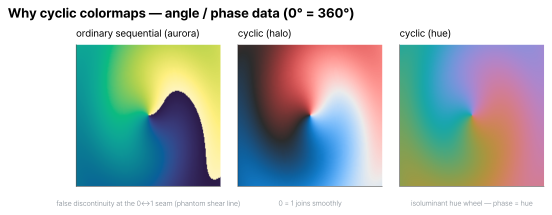
Angle and phase data (0° = 360° — CFD phase fields, FFT phase, wind direction) drawn with an ordinary sequential map grow a false discontinuity at the 0↔1 seam. A cyclic map’s generating path closes at that join. The stored LUT remains endpoint-exclusive, so its first and last entries are adjacent rather than identical.

halo and corona are dark-center, double-lobed modeled-relative-Y loops; only hue is an isoluminant hue wheel. Ordered-map monotonicity does not apply to cyclic maps; seam ΔEOK and topology gates do, while only hue has a relative_y-spread gate.

What this system does not guarantee

Stated plainly, per principle 4:

• Neutral-coordinate convergence in diverging maps. Both arms converge to the same center by design. In workflows that remove or alter color, use contours, hatching, or numbers alongside rather than relying on the palette alone.

• Bright-yellow text on white. No current shipped yellow token reaches 4.5:1 against white. Darker olive-yellow colors can exceed 4.5:1, but they are outside the shipped yellow ramp’s accepted endpoint. This is a selected-ramp identity choice, not a structural impossibility of yellow. It preserves the ramp’s accepted bright-yellow identity. Each family diagnostic card marks the first shipped step that passes its stated contrast check, or explicitly reports that no shipped step passes.

• Cross-family orthogonality of the warm dark steps. yellow9, amber9, and orange8 converge in a narrow hue corridor (a geometric consequence of the drift aesthetic); the family names’ color identity is reliable through steps 0–7.

• Display output or universal perceived brightness. Catalog relative_y is modeled from nominal sRGB values. It is neither a display measurement nor a complete appearance model; the Helmholtz–Kohlrausch effect can make a saturated color look brighter than a neutral with the same modeled Y.

• One contrast claim for every background. A WCAG contrast result applies only to its specified foreground/background pair. The dark preset’s seven-color cycle therefore has pair-specific WCAG text-contrast checks for named backgrounds and separate model-specific ΔE00/CVD collision diagnostics in src/dartwork_mpl/asset/mplstyle/theme-dark.mplstyle.

• Observer-wide accessibility. CIELAB/CIEDE2000 and the named CVD simulations are model-specific finished-output diagnostics. Their thresholds are regression contracts, not guarantees for an individual observer, viewing condition, or assistive need.

• turbo-style high-contrast rainbows. Non-monotonic modeled relative Y is a map property. Its suitability and its tendency to create ordering ambiguity or emphasize variation are task-dependent. That does not mean that all apparent detail is invented. iris keeps the accepted ordered-output topology across its wide hue path.

Reproducibility

The packaged v6 authority contains the palette-authoring recipe’s 107 named bookkeeping slots (116 scalar numeric leaves under the exclusions above), additional topology-specific continuous-map recipe data, compiled exact-output contracts, metric provenance, and catalog metadata. Historical v5 data remains an immutable compatibility fixture rather than a production recipe:

• docs/adr/0001-oklab-centered-color-construction.md — the accepted decision and rejected alternatives.

• src/dartwork_mpl/asset/color/color_v6_ssot.json — the packaged operational recipe and contract SSOT.

• docs/superpowers/specs/assets/2026-07-14-oklab-centered-color-system/ — the frozen v5 compatibility and quality fixtures.

• docs/color_system/generate_theory_figures.py — regenerates the figures above from the shipped package (run only when the SSOT changes).

See also

• Colors — the generated dc.* families as swatch sheets.

• Palettes — pick a cycle by intent.

• Colormaps — the 43-map catalog, applied.

• Color class — the Color class and custom colormaps.

Typography rationale

The font system now follows the same evidence pattern as color: families are not bundled because they look plausible in a specimen sheet.

Each family has one chart job. Every measured claim is derived from the shipped font files, and the fallback chain is treated as product behavior rather than an accident of matplotlib configuration.

T1 · Jobs before taste. Every registered matplotlib family has exactly one documented role: body, display, Korean body, serif, monospace, Korean monospace, or fallback tail. A new family must do a job that another bundled family does not already do better.

T2 · Measured gates. OS/2 weights, matplotlib-safe numeric axes, browser-only tabular-numeral availability, fixed-width truth, chart-glyph coverage, Hangul coverage, and license class are read from the bundled files in tests and docs. Known upstream metadata quirks are named in the registry instead of being silently normalized.

T3 · Roles in user space. Presets and docs speak in roles, while users keep native matplotlib Figure / Axes objects. Size and weight still flow through dm.fs() and dm.fw(), so swapping presets does not strand literal point sizes or arbitrary font weights.

T4 · Fallback is pinned. The base text chain is Roboto → Inter → Paperlogy → Noto Sans CJK KR → Pretendard → Noto Sans Math → Noto Sans Symbols → Noto Sans Symbols 2 → sans-serif. Tests pin the first family that resolves every guaranteed chart glyph, the digits, and 한.

Role	Default	Alternates	Job
body	Roboto	Inter · IBM Plex Sans · Source Sans 3 · Noto Sans	neutral Latin chart text and editorial alternates
display	Inter Display	-	large titles, headings, poster-scale numerals
kr-body	Paperlogy	Pretendard · Noto Sans CJK KR	Korean and CJK labels without system-font dependence
serif	Source Serif 4	-	opt-in serif body for journal- or book-matched figures (not in any preset chain)
mono	JetBrains Mono	IBM Plex Mono · Roboto Mono · Source Code Pro	code, timestamps, aligned labels, tabular data
mono-kr	D2Coding	-	monospaced Hangul for code blocks and aligned Korean tables
fallback-tail	Noto Sans Math	Noto Sans Symbols · Noto Sans Symbols 2	math operators, arrows, signs, and dingbats

Source Serif 4 is an opt-in family: it is not wired into any preset fallback chain, so a serif figure asks for it explicitly with plt.rcParams["font.family"] = "Source Serif 4".

No Korean serif (명조) is bundled — a legible Hangul serif would add several megabytes, so KR serif is out of scope by design.

For monospaced Hangul (code blocks, aligned Korean tables), set font.family = ["JetBrains Mono", "D2Coding"] so both scripts stay fixed-width.

Family	Role	Weights	Aligned digits	tnum available	Chart glyphs	Hangul	License
Roboto	body	100, 200, 300, 400, 500, 600, 700, 800, 900	digits	yes	7/8 −×±°μσΔ	-	OFL-1.1
Inter	body	100, 200, 300, 400, 500, 600, 700, 800, 900	-	yes	8/8 −×±→°μσΔ	-	OFL-1.1
IBM Plex Sans	body	100, 200, 300, 400, 500, 600, 700	digits	-	8/8 −×±→°μσΔ	-	OFL-1.1
Source Sans 3	body	200, 300, 400, 500, 600, 700, 900	digits	-	8/8 −×±→°μσΔ	-	OFL-1.1
Noto Sans	body	100, 200, 300, 400, 500, 600, 700, 800, 900	digits	yes	7/8 −×±°μσΔ	-	OFL-1.1
Inter Display	display	100, 200, 300, 400, 500, 600, 700, 800, 900	-	yes	8/8 −×±→°μσΔ	-	OFL-1.1
Paperlogy	kr-body	250, 300, 400, 500, 600, 700, 800, 900	digits	-	5/8 −×±→°	yes	OFL-1.1
Pretendard	kr-body	100, 200, 300, 400, 500, 600, 700, 800, 900	-	yes	8/8 −×±→°μσΔ	yes	OFL-1.1
Noto Sans CJK KR	kr-body	400	digits	-	3/8 ×±°	yes	OFL-1.1
Source Serif 4	serif	200, 300, 400, 600, 700, 900	digits	yes	8/8 −×±→°μσΔ	-	OFL-1.1
Noto Serif	serif	100, 200, 300, 400, 500, 600, 700, 800, 900	digits	yes	7/8 −×±°μσΔ	-	OFL-1.1
IBM Plex Serif	serif	100, 200, 300, 400, 500, 600, 700	digits	-	8/8 −×±→°μσΔ	-	OFL-1.1
JetBrains Mono	mono	100, 200, 300, 400, 500, 600, 700, 800	mono	-	8/8 −×±→°μσΔ	-	OFL-1.1
IBM Plex Mono	mono	100, 200, 300, 400, 500, 600, 700	mono	-	5/8 −×±→°	-	OFL-1.1
Roboto Mono	mono	100, 200, 300, 400, 500, 600, 700	mono	-	7/8 −×±°μσΔ	-	OFL-1.1
Source Code Pro	mono	200, 300, 400, 500, 600, 700, 900	mono	-	8/8 −×±→°μσΔ	-	OFL-1.1
D2Coding	mono-kr	400, 700	mono	-	8/8 −×±→°μσΔ	yes	OFL-1.1
Noto Sans Math	fallback-tail	400	digits	-	8/8 −×±→°μσΔ	-	OFL-1.1
Noto Sans Symbols	fallback-tail	400	digits	-	4/8 −×→°	-	OFL-1.1
Noto Sans Symbols 2	fallback-tail	400	digits	-	3/8 −×°	-	OFL-1.1

In the matrix, Aligned digits means the default digit advances are uniform in real matplotlib output, or the family is fixed-width.

tnum available is a browser/specimen signal only: Inter and Pretendard expose the OpenType feature, but matplotlib does not apply it. Use IBM Plex Sans, Source Sans 3, Paperlogy, Noto Sans, Roboto, Source Serif 4, or monospace families when aligned numeric axes are the requirement.

Anatomy of the fallback chain

Plain text in matplotlib resolves glyphs from font.family, so the chain must name actual bundled families, not just the generic sans-serif alias.

The order starts with the body voice (Roboto, then Inter), moves through Korean and CJK coverage (Paperlogy, Noto Sans CJK KR, Pretendard), then lands on math and symbol faces.

In the pinned resolver map, digits and most operators resolve in Roboto, → first appears in Inter, and 한 first appears in Paperlogy; nothing falls through to DejaVu.

font.sans-serif is held identical to font.family — bundled families plus the generic terminator, with no machine-dependent OS fonts (Lato, Arial, Malgun Gothic, …). Anything past the bundle intentionally falls to matplotlib’s default rather than a font that happens to be installed. Byte reproducibility is bounded to bundled glyph coverage and a pinned rendering environment; unpinned matplotlib, FreeType, backend, or missing-glyph behavior can still change output.

Math segments obey the same discipline. The custom mathtext fontset is matched to the body: rm/it/bf/sf are Roboto, tt is JetBrains Mono, and cal is the matplotlib-bundled STIXGeneral.

Greek and operators absent from those fall to stixsans (also matplotlib-bundled), never DejaVu. mathtext.default: regular makes a bare $R^2$ render in the same upright body face as the labels around it.

Under a -kr preset the body face is Paperlogy, so the Latin and digits in a math span match the Korean labels while symbols still resolve through STIX.