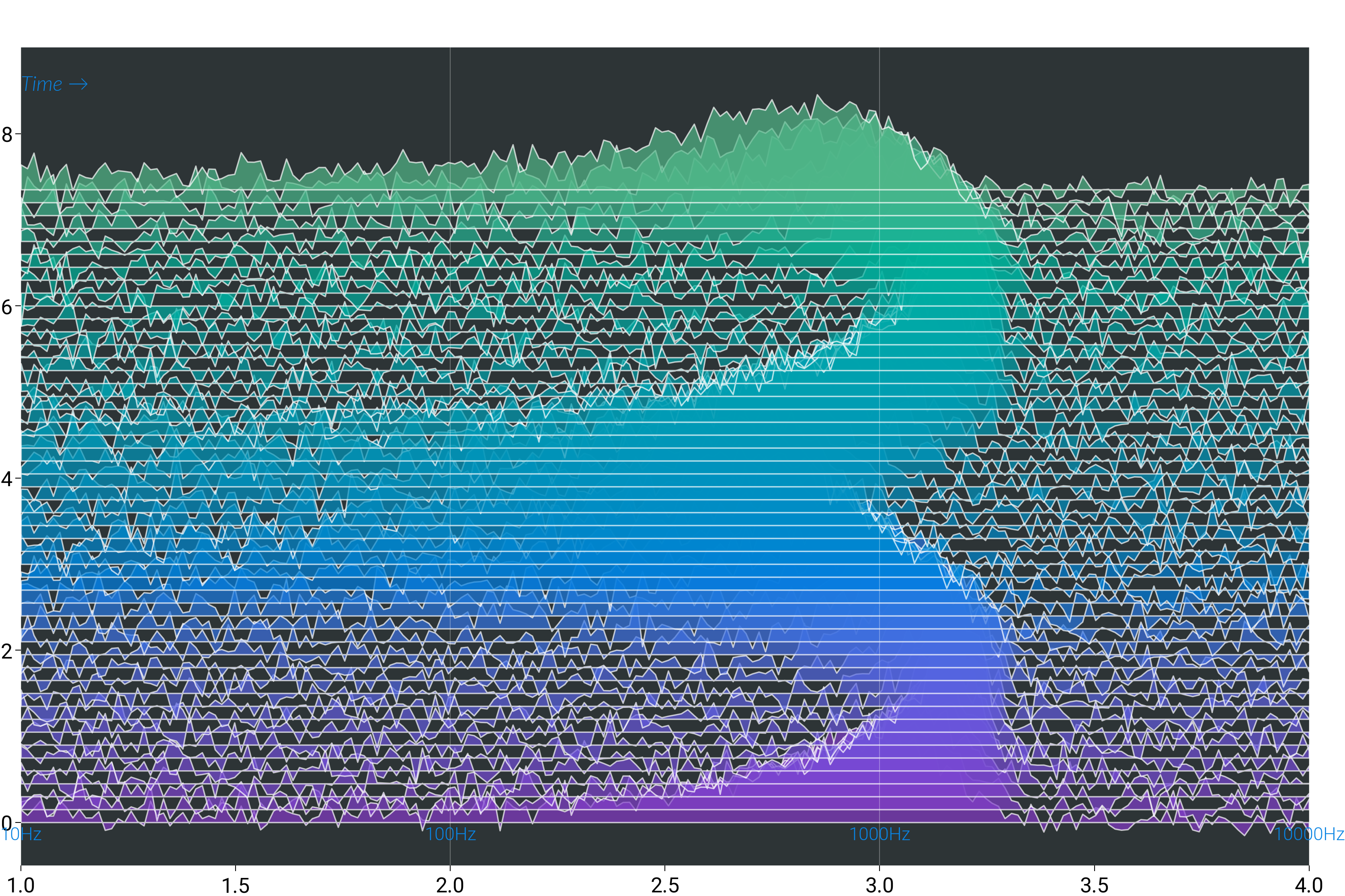
Frequency Response Waterfall

A pseudo-3D waterfall of evolving frequency responses. Each time slice is plotted as a filled curve in log-frequency space, offset vertically to suggest depth. The colour ramp moves along the time axis using a purple-to-green dm.cspace gradient.

Practical points:

• Frequencies are placed on a log scale via np.logspace and rendered against np.log10(freq) for control over tick placement.

• Vertical offsets (y_offset = i * 0.15) create the staircase effect without needing a real 3D axes.

import matplotlib.pyplot as plt
import numpy as np

import dartwork_mpl as dm

np.random.seed(42)
dm.style.use("scientific")

fig, ax = plt.subplots(figsize=dm.figsize("17cm", "wide"))

n_time_steps = 50
n_frequencies = 200
time = np.linspace(0, 10, n_time_steps)
freq = np.logspace(1, 4, n_frequencies)  # 10Hz to 10kHz

responses = []
for t in time:
    center_freq = 1000 * (1 + 0.5 * np.sin(t))
    bandwidth = 500 * (1 + 0.3 * np.cos(2 * t))
    response = np.exp(-(((freq - center_freq) / bandwidth) ** 2))
    response += 0.1 * np.random.randn(n_frequencies)
    responses.append(response)

waterfall_colors = dm.cspace("oc.purple8", "dc.forest2", n=n_time_steps)

for i, response in enumerate(responses):
    color = waterfall_colors[i]
    y_offset = i * 0.15
    ax.fill_between(
        np.log10(freq),
        y_offset,
        response + y_offset,
        color=color.to_hex(),
        alpha=0.7,
        edgecolor="white",
        linewidth=0.5,
    )

for f in [10, 100, 1000, 10000]:
    ax.axvline(np.log10(f), color="white", lw=0.3, alpha=0.3)
    ax.text(
        np.log10(f),
        -0.2,
        f"{f}Hz",
        ha="center",
        fontsize=dm.fs(-1),
        color="dc.nordic2",
    )

ax.set_xlim(1, 4)
ax.set_ylim(-0.5, n_time_steps * 0.15 + 1.5)
for s in ax.spines.values():
    s.set_visible(False)
ax.set_facecolor("dc.nordic5")

ax.text(
    2.5,
    n_time_steps * 0.15 + 1.8,
    "Frequency Response Evolution",
    ha="center",
    fontsize=dm.fs(3),
    color="white",
    weight="bold",
)
ax.text(
    1,
    n_time_steps * 0.15 + 1,
    "Time →",
    fontsize=dm.fs(0),
    color="dc.nordic2",
    style="italic",
)

dm.simple_layout(fig)
plt.show()