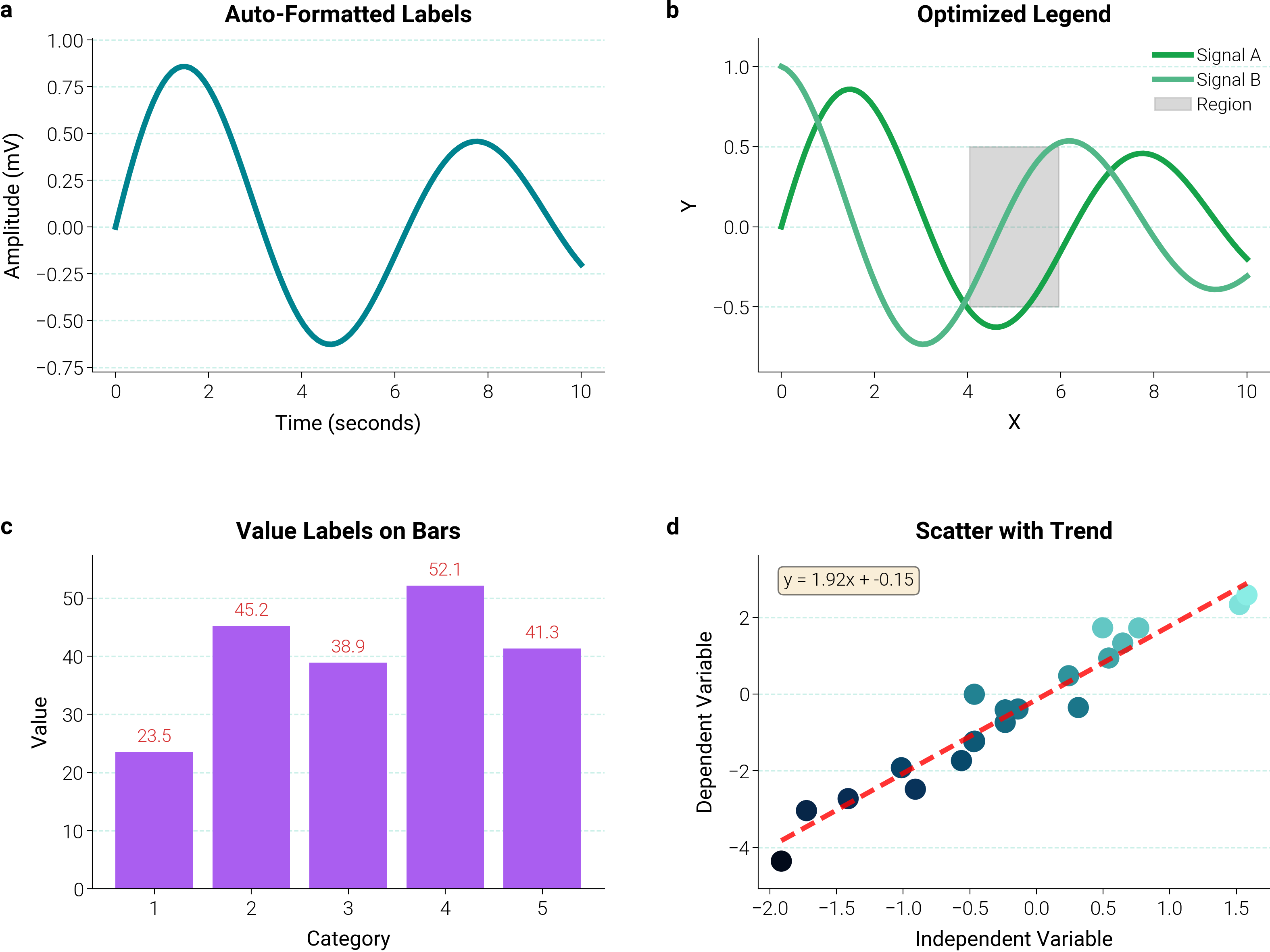
helpers.labels — Legend and Value Annotations

dm.helpers.labels provides optimize_legend for smart legend placement and add_value_labels (now inlined) for per-point numeric annotations. Axis labels are set directly via ax.set_xlabel / ax.set_ylabel.

The 2×2 grid below shows each pattern on synthetic data.

import matplotlib.pyplot as plt
import numpy as np

import dartwork_mpl as dm


def _minimal(ax: plt.Axes) -> None:
    """Inline minimal-axes recipe (top/right hidden + light dashed y-grid)."""
    ax.spines["top"].set_visible(False)
    ax.spines["right"].set_visible(False)
    ax.grid(
        True,
        axis="y",
        alpha=0.2,
        color="dc.nordic1",
        linestyle="--",
        linewidth=0.5,
    )
    ax.set_axisbelow(True)


np.random.seed(42)

dm.style.use("scientific")
fig, axes = plt.subplots(
    2,
    2,
    figsize=dm.figsize("16cm", "standard"),
    gridspec_kw={"hspace": 0.55, "wspace": 0.3},
)

x = np.linspace(0, 10, 100)
y1 = np.sin(x) * np.exp(-x / 10)
y2 = np.cos(x) * np.exp(-x / 10)

# Format axis labels from name + unit.
ax1 = axes[0, 0]
ax1.plot(x, y1, color="dc.ocean2", lw=dm.lw(1))
ax1.set_xlabel("Time (seconds)", fontsize=dm.fs(0))
ax1.set_ylabel("Amplitude (mV)", fontsize=dm.fs(0))
ax1.set_title("Auto-Formatted Labels", fontsize=dm.fs(1))
_minimal(ax1)

# Optimized legend placement.
ax2 = axes[0, 1]
ax2.plot(x, y1, color="dc.vivid2", label="Signal A", lw=dm.lw(1))
ax2.plot(x, y2, color="dc.forest2", label="Signal B", lw=dm.lw(1))
ax2.fill_between(x[40:60], -0.5, 0.5, alpha=0.3, color="gray", label="Region")
dm.helpers.labels.optimize_legend(ax2, preferred_loc="best")
ax2.set_title("Optimized Legend", fontsize=dm.fs(1))
ax2.set_xlabel("X", fontsize=dm.fs(0))
ax2.set_ylabel("Y", fontsize=dm.fs(0))
_minimal(ax2)

# Value labels above bars.
ax3 = axes[1, 0]
x_points = np.array([1, 2, 3, 4, 5])
y_points = np.array([23.5, 45.2, 38.9, 52.1, 41.3])
ax3.bar(x_points, y_points, color="oc.purple5")
y_min, y_max = ax3.get_ylim()
_offset = (y_max - y_min) * 0.02
for xi, yi in zip(x_points, y_points, strict=False):
    ax3.text(
        xi,
        yi + _offset,
        f"{yi:.1f}",
        ha="center",
        va="bottom",
        fontsize=dm.fs(-1),
        color="dc.nordic3",
    )
ax3.set_title("Value Labels on Bars", fontsize=dm.fs(1))
ax3.set_xlabel("Category", fontsize=dm.fs(0))
ax3.set_ylabel("Value", fontsize=dm.fs(0))
_minimal(ax3)

# Scatter with a fitted trend line and regression-equation annotation.
ax4 = axes[1, 1]
x_scatter = np.random.randn(20)
y_scatter = 2 * x_scatter + np.random.randn(20) * 0.5
ax4.scatter(x_scatter, y_scatter, c=y_scatter, cmap="dc.deep_sea", s=50)
ax4.set_xlabel("Independent Variable", fontsize=dm.fs(0))
ax4.set_ylabel("Dependent Variable", fontsize=dm.fs(0))
z = np.polyfit(x_scatter, y_scatter, 1)
p = np.poly1d(z)
x_trend = np.linspace(x_scatter.min(), x_scatter.max(), 100)
ax4.plot(x_trend, p(x_trend), "r--", alpha=0.8, lw=dm.lw(0.8))
ax4.text(
    0.05,
    0.95,
    f"y = {z[0]:.2f}x + {z[1]:.2f}",
    transform=ax4.transAxes,
    fontsize=dm.fs(-1),
    verticalalignment="top",
    bbox={"boxstyle": "round", "facecolor": "wheat", "alpha": 0.5},
)
ax4.set_title("Scatter with Trend", fontsize=dm.fs(1))
_minimal(ax4)

dm.label_axes(axes.flat)
dm.simple_layout(fig)
plt.show()