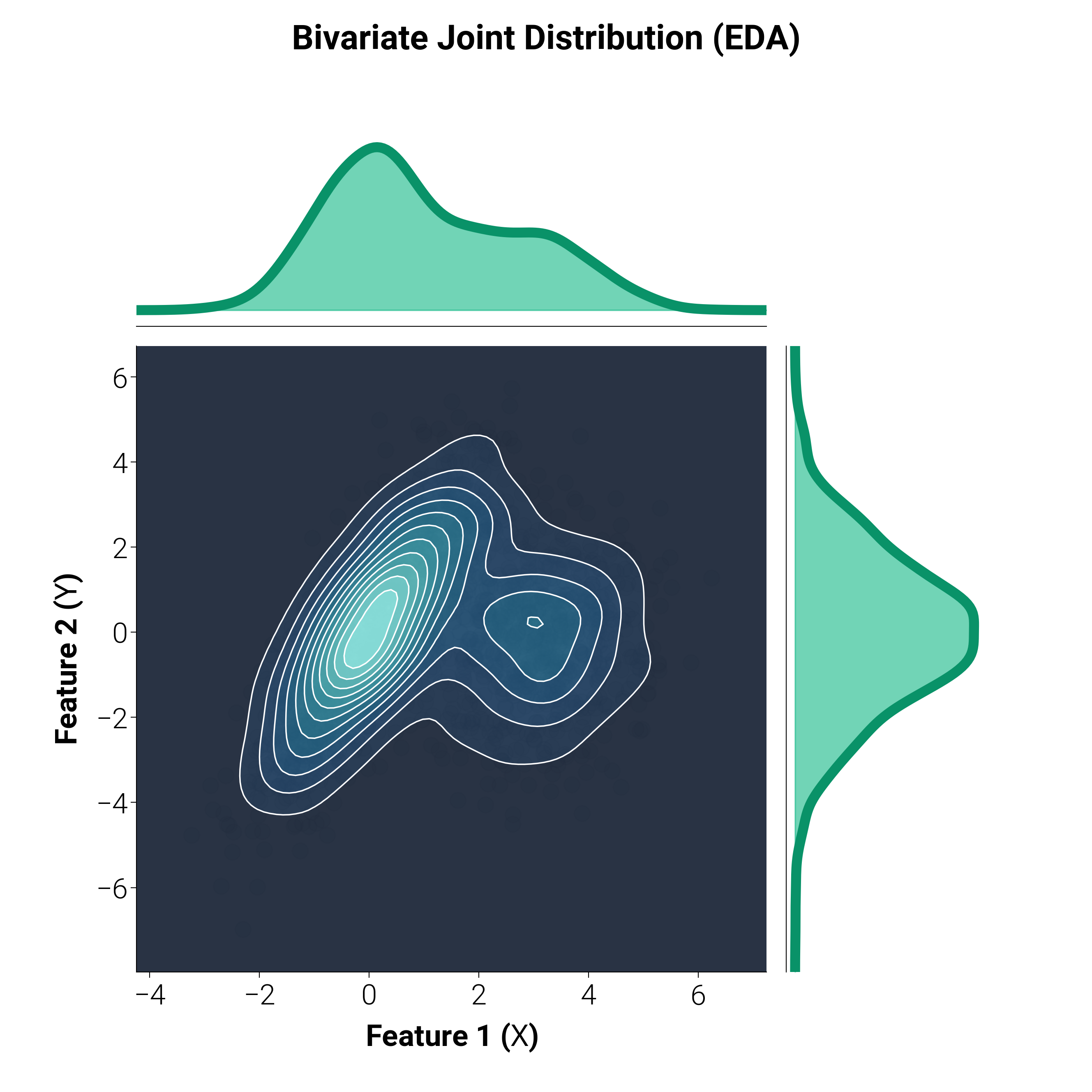
Bivariate KDE with Marginals

A staple of Exploratory Data Analysis (EDA) in Data Science. This plot shows the joint distribution of two continuous variables using a 2D kernel density estimate (KDE) and contour plot, flanked by their 1D marginal distributions.

We construct this layout manually using matplotlib.gridspec to demonstrate how dartwork-mpl’s styling seamlessly integrates with complex, tightly coupled subplots.

import matplotlib.gridspec as gridspec
import matplotlib.pyplot as plt
import numpy as np
from scipy.stats import gaussian_kde

import dartwork_mpl as dm

dm.style.use("presentation")

np.random.seed(42)

# Generate correlated bivariate data
n = 1500
x = np.random.normal(0, 1, n)
y = 1.5 * x + np.random.normal(0, 1.2, n)
# add a second cluster
x = np.concatenate([x, np.random.normal(3, 1, n // 2)])
y = np.concatenate([y, np.random.normal(0, 1.5, n // 2)])

fig = plt.figure(figsize=(dm.SW * 1.5, dm.SW * 1.5))
gs = gridspec.GridSpec(4, 4, figure=fig, hspace=0.1, wspace=0.1)

# Main joint plot (contour)
ax_joint = fig.add_subplot(gs[1:4, 0:3])
# Top marginal (histogram/density)
ax_marg_x = fig.add_subplot(gs[0, 0:3], sharex=ax_joint)
# Right marginal (histogram/density)
ax_marg_y = fig.add_subplot(gs[1:4, 3], sharey=ax_joint)

# 1. Plot the joint 2D KDE
xmin, xmax = x.min() - 1, x.max() + 1
ymin, ymax = y.min() - 1, y.max() + 1
X, Y = np.mgrid[xmin:xmax:100j, ymin:ymax:100j]
positions = np.vstack([X.ravel(), Y.ravel()])
values = np.vstack([x, y])
kernel = gaussian_kde(values)
Z = np.reshape(kernel(positions).T, X.shape)

# Base scatter for context, contour for density
ax_joint.scatter(x, y, s=dm.fs(-5) ** 2, color="oc.gray5", alpha=0.1, zorder=1)
contour = ax_joint.contourf(
    X, Y, Z, levels=12, cmap="dc.deep_sea", alpha=0.85, zorder=2
)
ax_joint.contour(X, Y, Z, levels=12, colors="white", linewidths=0.5, zorder=3)

# 2. Plot the marginal distributions
cm_color = dm.named("oc.teal6")

# Marginal X
x_eval = np.linspace(xmin, xmax, 200)
kde_x = gaussian_kde(x)(x_eval)
ax_marg_x.fill_between(x_eval, 0, kde_x, color=cm_color.to_hex(), alpha=0.6)
ax_marg_x.plot(x_eval, kde_x, color="oc.teal8", lw=dm.lw(2.5))

# Marginal Y
y_eval = np.linspace(ymin, ymax, 200)
kde_y = gaussian_kde(y)(y_eval)
ax_marg_y.fill_betweenx(y_eval, 0, kde_y, color=cm_color.to_hex(), alpha=0.6)
ax_marg_y.plot(kde_y, y_eval, color="oc.teal8", lw=dm.lw(2.5))

# 3. Cleanup axes and layout
for spine in ["top", "right", "left"]:
    ax_marg_x.spines[spine].set_visible(False)
ax_marg_x.set_yticks([])
ax_marg_x.tick_params(labelbottom=False, bottom=False)

for spine in ["top", "right", "bottom"]:
    ax_marg_y.spines[spine].set_visible(False)
ax_marg_y.set_xticks([])
ax_marg_y.tick_params(labelleft=False, left=False)

ax_joint.set_xlabel("Feature 1 ($X$)", fontsize=dm.fs(0), weight="bold")
ax_joint.set_ylabel("Feature 2 ($Y$)", fontsize=dm.fs(0), weight="bold")
dm.set_decimal(ax_joint)

fig.suptitle(
    "Bivariate Joint Distribution (EDA)",
    fontsize=dm.fs(1.5),
    weight="bold",
    y=0.98,
)

# Because we manually tight-packed the gridspec, we don't automatically call tight_layout
# or if we do, we need to respect the GridSpec layout.
# simple_layout can disrupt finely tuned GridSpecs.
plt.show()