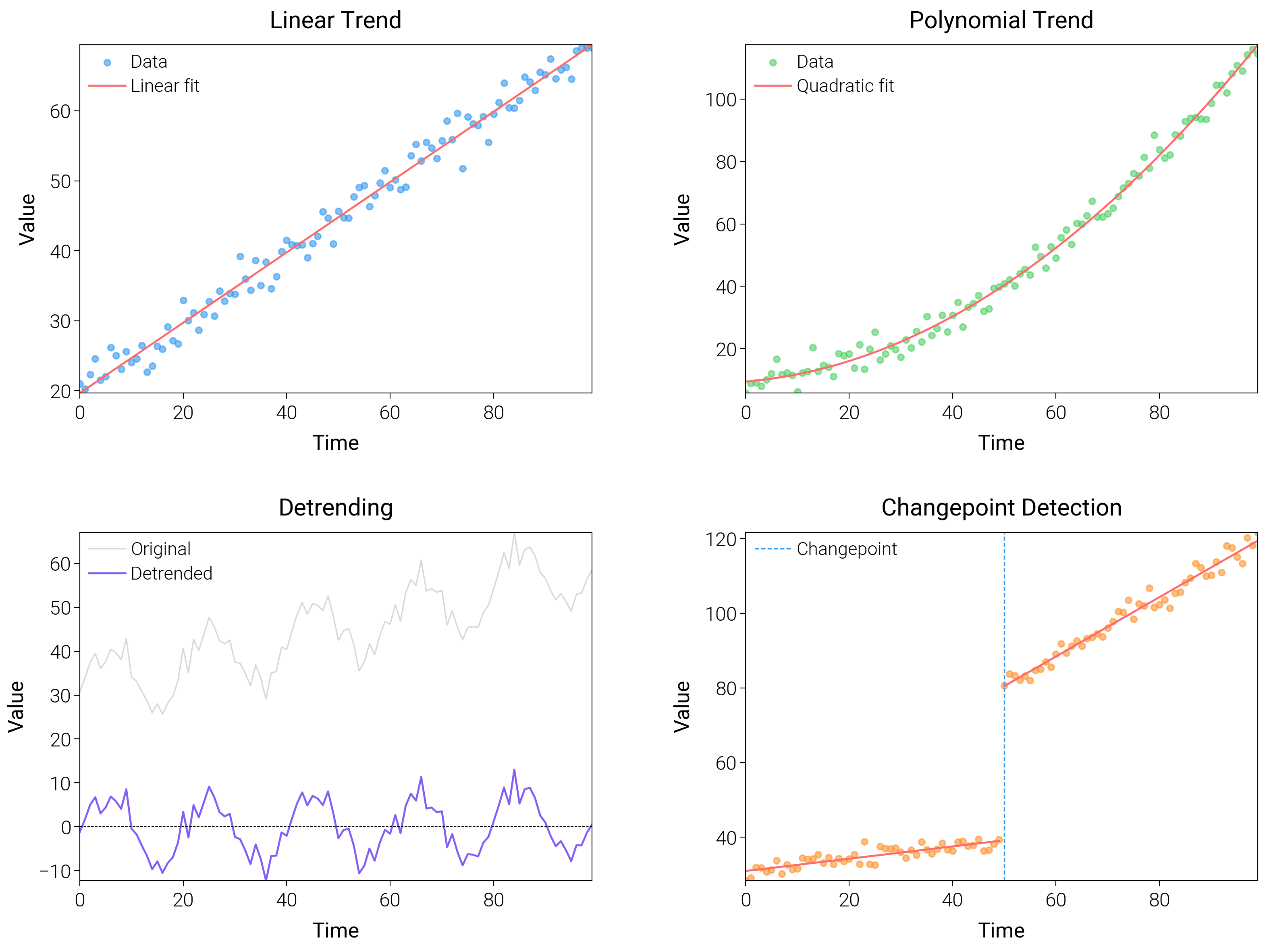
Trend Analysis

Highlight local and global trends with smoothing, break annotations, and slope callouts.

import matplotlib.pyplot as plt
import numpy as np

import dartwork_mpl as dm

dm.style.use("scientific")

# Generate time series with different trends
np.random.seed(42)
n = 100
t = np.arange(n)

# Linear trend
linear_trend = 20 + 0.5 * t + np.random.randn(n) * 2

# Quadratic trend
quad_trend = 10 + 0.1 * t + 0.01 * t**2 + np.random.randn(n) * 3

# Seasonal + trend
seasonal_trend = (
    30 + 0.3 * t + 8 * np.sin(2 * np.pi * t / 20) + np.random.randn(n) * 2
)

# Changepoint
change_trend = (
    np.concatenate([30 + 0.2 * t[:50], 40 + 0.8 * t[50:]])
    + np.random.randn(n) * 2
)

fig = plt.figure(figsize=(dm.cm2in(16), dm.cm2in(12)), dpi=300)
gs = fig.add_gridspec(
    nrows=2,
    ncols=2,
    left=0.08,
    right=0.98,
    top=0.95,
    bottom=0.08,
    wspace=0.3,
    hspace=0.4,
)

# Panel A: Linear trend
ax1 = fig.add_subplot(gs[0, 0])
ax1.scatter(t, linear_trend, c="oc.blue5", s=5, alpha=0.6, label="Data")
z = np.polyfit(t, linear_trend, 1)
p = np.poly1d(z)
ax1.plot(t, p(t), color="oc.red5", lw=0.7, label="Linear fit")
ax1.set_xlabel("Time", fontsize=dm.fs(0))
ax1.set_ylabel("Value", fontsize=dm.fs(0))
ax1.set_title("Linear Trend", fontsize=dm.fs(1))
ax1.legend(loc="best", fontsize=dm.fs(-1))

# Panel B: Polynomial trend
ax2 = fig.add_subplot(gs[0, 1])
ax2.scatter(t, quad_trend, c="oc.green5", s=5, alpha=0.6, label="Data")
z2 = np.polyfit(t, quad_trend, 2)
p2 = np.poly1d(z2)
ax2.plot(t, p2(t), color="oc.red5", lw=0.7, label="Quadratic fit")
ax2.set_xlabel("Time", fontsize=dm.fs(0))
ax2.set_ylabel("Value", fontsize=dm.fs(0))
ax2.set_title("Polynomial Trend", fontsize=dm.fs(1))
ax2.legend(loc="best", fontsize=dm.fs(-1))

# Panel C: Detrending
ax3 = fig.add_subplot(gs[1, 0])
z3 = np.polyfit(t, seasonal_trend, 1)
p3 = np.poly1d(z3)
detrended = seasonal_trend - p3(t)
ax3.plot(
    t, seasonal_trend, color="oc.gray5", lw=0.5, alpha=0.5, label="Original"
)
ax3.plot(t, detrended, color="oc.violet5", lw=0.7, label="Detrended")
ax3.axhline(y=0, color="k", lw=0.3, linestyle="--")
ax3.set_xlabel("Time", fontsize=dm.fs(0))
ax3.set_ylabel("Value", fontsize=dm.fs(0))
ax3.set_title("Detrending", fontsize=dm.fs(1))
ax3.legend(loc="best", fontsize=dm.fs(-1))

# Panel D: Changepoint detection
ax4 = fig.add_subplot(gs[1, 1])
ax4.scatter(t, change_trend, c="oc.orange5", s=5, alpha=0.6)
# Fit two segments
z4a = np.polyfit(t[:50], change_trend[:50], 1)
z4b = np.polyfit(t[50:], change_trend[50:], 1)
p4a = np.poly1d(z4a)
p4b = np.poly1d(z4b)
ax4.plot(t[:50], p4a(t[:50]), color="oc.red5", lw=0.7)
ax4.plot(t[50:], p4b(t[50:]), color="oc.red5", lw=0.7)
ax4.axvline(x=50, color="oc.blue5", lw=0.5, linestyle="--", label="Changepoint")
ax4.set_xlabel("Time", fontsize=dm.fs(0))
ax4.set_ylabel("Value", fontsize=dm.fs(0))
ax4.set_title("Changepoint Detection", fontsize=dm.fs(1))
ax4.legend(loc="best", fontsize=dm.fs(-1))

dm.simple_layout(fig, gs=gs)
plt.show()