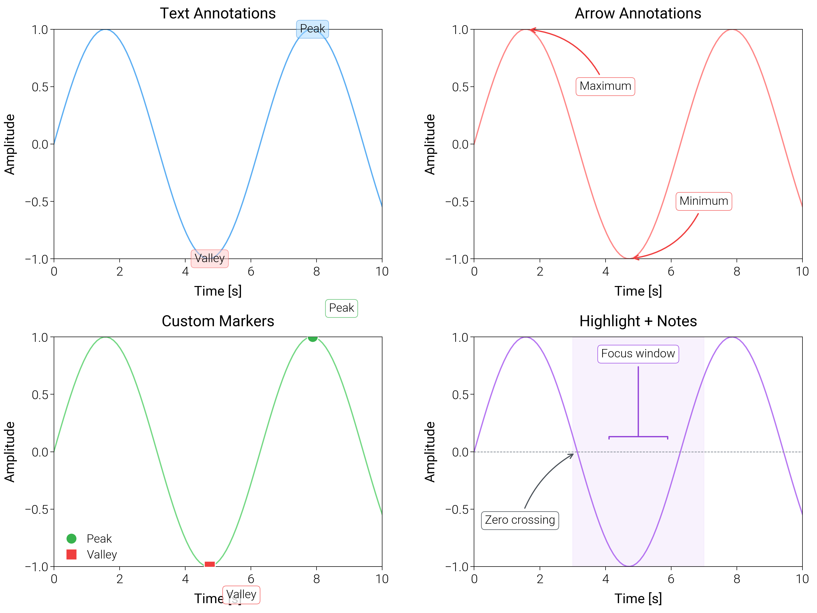
Annotations

Grab-and-go annotation snippets: arrows, text boxes, highlights, and callouts aligned to data or axes coords.

/home/runner/work/dartwork-mpl/dartwork-mpl/docs/examples_source/layout_styling/plot_annotations.py:199: UserWarning: Setting the 'color' property will override the edgecolor or facecolor properties.
  ax4.axvspan(

import matplotlib.pyplot as plt
import numpy as np

import dartwork_mpl as dm

# Apply scientific style preset
# Default: font.size=7.5, lines.linewidth=0.5, axes.linewidth=0.3
dm.style.use("scientific")

# Generate sample data
x = np.linspace(0, 10, 100)
y = np.sin(x)

# Create figure (2 x 2 layout, with generous top/bottom margins)
fig = plt.figure(figsize=(dm.cm2in(16), dm.cm2in(12)), dpi=300)
gs = fig.add_gridspec(
    nrows=2,
    ncols=2,
    left=0.08,
    right=0.98,
    top=0.93,
    bottom=0.12,
    wspace=0.28,
    hspace=0.34,
)

# Panel A: Text annotations
ax1 = fig.add_subplot(gs[0, 0])
ax1.plot(x, y, color="oc.blue5", lw=0.7, alpha=0.8)
# Text annotation: fontsize=dm.fs(-1), bbox with explicit parameters
peak_x = x[np.argmax(y)]
valley_x = x[np.argmin(y)]
ax1.text(
    peak_x,
    np.sin(peak_x),
    "Peak",
    fontsize=dm.fs(-1),
    bbox={
        "boxstyle": "round",
        "facecolor": "oc.blue2",
        "alpha": 0.5,
        "edgecolor": "oc.blue7",
        "linewidth": 0.3,
    },
    ha="center",
    va="center",
)
ax1.text(
    valley_x,
    np.sin(valley_x),
    "Valley",
    fontsize=dm.fs(-1),
    bbox={
        "boxstyle": "round",
        "facecolor": "oc.red2",
        "alpha": 0.5,
        "edgecolor": "oc.red7",
        "linewidth": 0.3,
    },
    ha="center",
    va="center",
)
ax1.set_xlabel("Time [s]", fontsize=dm.fs(0))
ax1.set_ylabel("Amplitude", fontsize=dm.fs(0))
ax1.set_title("Text Annotations", fontsize=dm.fs(1))
ax1.set_xticks([0, 2, 4, 6, 8, 10])
ax1.set_yticks([-1, -0.5, 0, 0.5, 1])

# Panel B: Arrow annotations
ax2 = fig.add_subplot(gs[0, 1])
ax2.plot(x, y, color="oc.red5", lw=0.7, alpha=0.8)
# Arrow annotation: arrowprops with explicit parameters
ax2.annotate(
    "Maximum",
    xy=(np.pi / 2, 1),
    xytext=(4, 0.5),
    arrowprops={
        "arrowstyle": "->",
        "color": "oc.red7",
        "lw": 0.7,
        "connectionstyle": "arc3,rad=0.3",
    },
    fontsize=dm.fs(-1),
    ha="center",
    va="center",
    bbox={
        "boxstyle": "round",
        "facecolor": "white",
        "alpha": 0.8,
        "edgecolor": "oc.red7",
        "linewidth": 0.3,
    },
)
ax2.annotate(
    "Minimum",
    xy=(3 * np.pi / 2, -1),
    xytext=(7, -0.5),
    arrowprops={
        "arrowstyle": "->",
        "color": "oc.red7",
        "lw": 0.7,
        "connectionstyle": "arc3,rad=-0.3",
    },
    fontsize=dm.fs(-1),
    ha="center",
    va="center",
    bbox={
        "boxstyle": "round",
        "facecolor": "white",
        "alpha": 0.8,
        "edgecolor": "oc.red7",
        "linewidth": 0.3,
    },
)
ax2.set_xlabel("Time [s]", fontsize=dm.fs(0))
ax2.set_ylabel("Amplitude", fontsize=dm.fs(0))
ax2.set_title("Arrow Annotations", fontsize=dm.fs(1))
ax2.set_xticks([0, 2, 4, 6, 8, 10])
ax2.set_yticks([-1, -0.5, 0, 0.5, 1])

# Panel C: Custom markers with labels
ax3 = fig.add_subplot(gs[1, 0])
ax3.plot(x, y, color="oc.green5", lw=0.7, alpha=0.8)
# Mark specific points: markersize=6, markeredgewidth=0.5
peak_idx = np.argmax(y)
valley_idx = np.argmin(y)
ax3.plot(
    x[peak_idx],
    y[peak_idx],
    "o",
    color="oc.green7",
    markersize=6,
    markeredgewidth=0.5,
    markeredgecolor="white",
    label="Peak",
    zorder=5,
)
ax3.plot(
    x[valley_idx],
    y[valley_idx],
    "s",
    color="oc.red7",
    markersize=6,
    markeredgewidth=0.5,
    markeredgecolor="white",
    label="Valley",
    zorder=5,
)
# Add labels next to markers: fontsize=dm.fs(-1)
ax3.text(
    x[peak_idx] + 0.5,
    y[peak_idx] + 0.2,
    "Peak",
    fontsize=dm.fs(-1),
    ha="left",
    va="bottom",
    bbox={
        "boxstyle": "round",
        "facecolor": "white",
        "alpha": 0.8,
        "edgecolor": "oc.green7",
        "linewidth": 0.3,
    },
)
ax3.text(
    x[valley_idx] + 0.5,
    y[valley_idx] - 0.2,
    "Valley",
    fontsize=dm.fs(-1),
    ha="left",
    va="top",
    bbox={
        "boxstyle": "round",
        "facecolor": "white",
        "alpha": 0.8,
        "edgecolor": "oc.red7",
        "linewidth": 0.3,
    },
)
ax3.set_xlabel("Time [s]", fontsize=dm.fs(0))
ax3.set_ylabel("Amplitude", fontsize=dm.fs(0))
ax3.set_title("Custom Markers", fontsize=dm.fs(1))
ax3.legend(loc="best", fontsize=dm.fs(-1), ncol=1)
ax3.set_xticks([0, 2, 4, 6, 8, 10])
ax3.set_yticks([-1, -0.5, 0, 0.5, 1])

# Panel D: Highlighted spans with inline notes
ax4 = fig.add_subplot(gs[1, 1])
ax4.plot(x, y, color="oc.purple5", lw=0.7, alpha=0.85)
ax4.axhline(0, color="oc.gray6", lw=0.4, linestyle="--")
# Highlight a time window
ax4.axvspan(
    3, 7, color="oc.purple1", alpha=0.35, edgecolor="oc.purple6", lw=0.4
)
ax4.annotate(
    "Focus window",
    xy=(5, 0.1),
    xytext=(5, 0.85),
    ha="center",
    va="center",
    fontsize=dm.fs(-1),
    arrowprops={
        "arrowstyle": "-[,widthB=2.5",
        "lw": 0.7,
        "color": "oc.purple7",
    },
    bbox={
        "boxstyle": "round",
        "facecolor": "white",
        "edgecolor": "oc.purple6",
        "linewidth": 0.3,
    },
)
ax4.annotate(
    "Zero crossing",
    xy=(np.pi, 0),
    xytext=(1.4, -0.6),
    fontsize=dm.fs(-1),
    ha="center",
    va="center",
    arrowprops={
        "arrowstyle": "->",
        "lw": 0.6,
        "color": "oc.gray7",
        "connectionstyle": "arc3,rad=-0.2",
    },
    bbox={
        "boxstyle": "round",
        "facecolor": "white",
        "edgecolor": "oc.gray7",
        "linewidth": 0.3,
    },
)
ax4.set_xlabel("Time [s]", fontsize=dm.fs(0))
ax4.set_ylabel("Amplitude", fontsize=dm.fs(0))
ax4.set_title("Highlight + Notes", fontsize=dm.fs(1))
ax4.set_xticks([0, 2, 4, 6, 8, 10])
ax4.set_yticks([-1, -0.5, 0, 0.5, 1])

# Optimize layout
dm.simple_layout(fig, gs=gs)

# Show plot
plt.show()