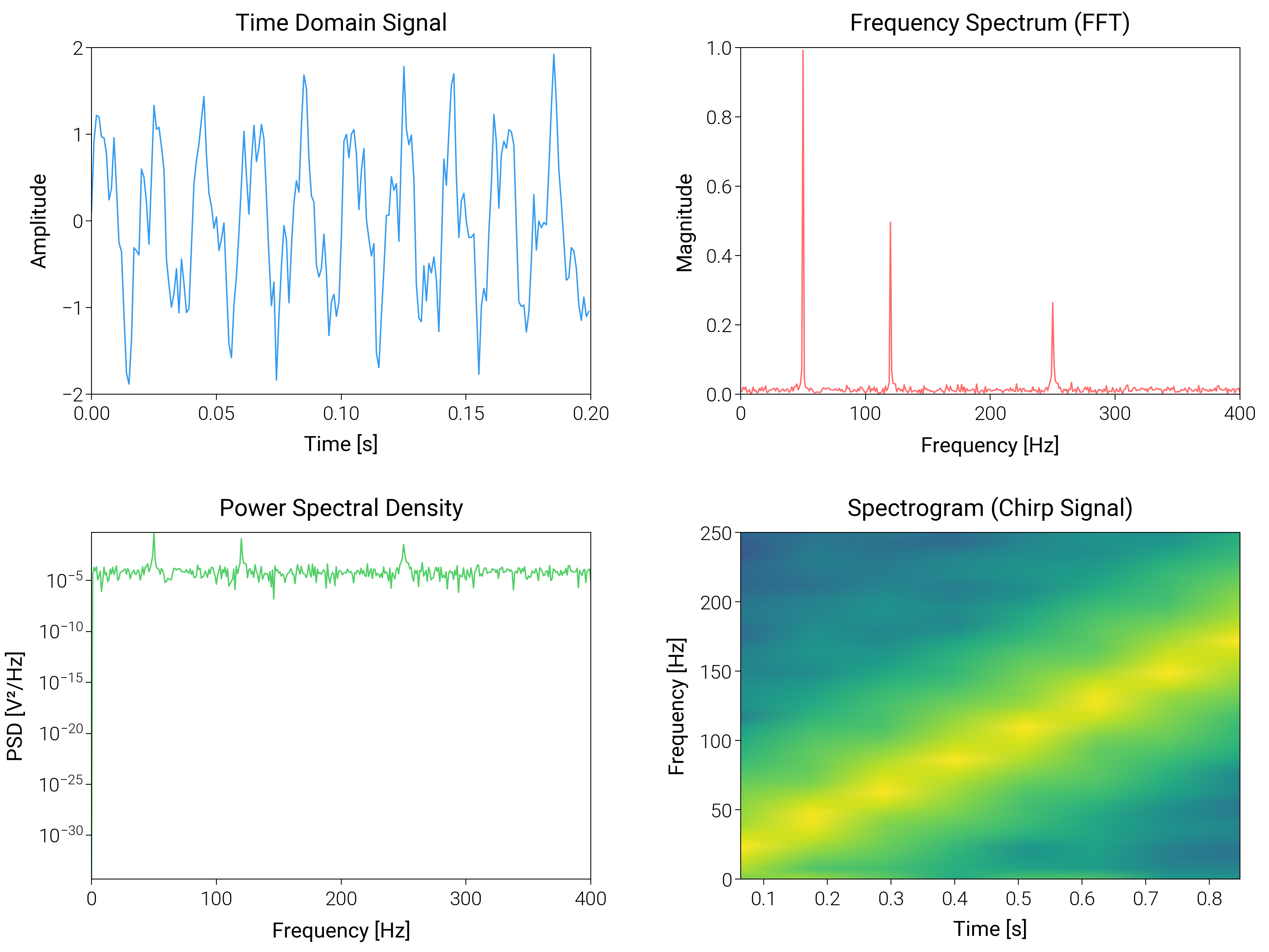
Spectral Analysis

Move from signals to frequency domain with windows, PSDs, spectrograms, and labelled peaks.

import matplotlib.pyplot as plt
import numpy as np
from scipy import signal

import dartwork_mpl as dm

# Apply scientific style preset
dm.style.use("scientific")

# Generate signals
np.random.seed(42)
fs = 1000  # Sampling frequency
t = np.linspace(0, 1, fs)
# Signal with multiple frequencies
f1, f2, f3 = 50, 120, 250
signal1 = (
    np.sin(2 * np.pi * f1 * t)
    + 0.5 * np.sin(2 * np.pi * f2 * t)
    + 0.3 * np.sin(2 * np.pi * f3 * t)
)
signal_noisy = signal1 + 0.2 * np.random.randn(len(t))

# Create figure
fig = plt.figure(figsize=(dm.cm2in(16), dm.cm2in(12)), dpi=300)

# Create GridSpec for 2x2 subplots
gs = fig.add_gridspec(
    nrows=2,
    ncols=2,
    left=0.08,
    right=0.98,
    top=0.95,
    bottom=0.08,
    wspace=0.3,
    hspace=0.4,
)

# Panel A: Time domain signal
ax1 = fig.add_subplot(gs[0, 0])
ax1.plot(t[:200], signal_noisy[:200], color="oc.blue5", lw=0.5)
ax1.set_xlabel("Time [s]", fontsize=dm.fs(0))
ax1.set_ylabel("Amplitude", fontsize=dm.fs(0))
ax1.set_title("Time Domain Signal", fontsize=dm.fs(1))
ax1.set_xticks([0, 0.05, 0.1, 0.15, 0.2])
ax1.set_yticks([-2, -1, 0, 1, 2])

# Panel B: Fourier transform
ax2 = fig.add_subplot(gs[0, 1])
fft_vals = np.fft.fft(signal_noisy)
fft_freq = np.fft.fftfreq(len(signal_noisy), 1 / fs)
positive_freq = fft_freq[: len(fft_freq) // 2]
magnitude = 2 * np.abs(fft_vals[: len(fft_vals) // 2]) / len(signal_noisy)
ax2.plot(positive_freq, magnitude, color="oc.red5", lw=0.5)
ax2.set_xlabel("Frequency [Hz]", fontsize=dm.fs(0))
ax2.set_ylabel("Magnitude", fontsize=dm.fs(0))
ax2.set_title("Frequency Spectrum (FFT)", fontsize=dm.fs(1))
ax2.set_xlim(0, 400)
ax2.set_xticks([0, 100, 200, 300, 400])
ax2.set_yticks([0, 0.2, 0.4, 0.6, 0.8, 1.0])

# Panel C: Power spectral density
ax3 = fig.add_subplot(gs[1, 0])
f_psd, psd = signal.periodogram(signal_noisy, fs)
ax3.semilogy(f_psd, psd, color="oc.green5", lw=0.5)
ax3.set_xlabel("Frequency [Hz]", fontsize=dm.fs(0))
ax3.set_ylabel("PSD [V²/Hz]", fontsize=dm.fs(0))
ax3.set_title("Power Spectral Density", fontsize=dm.fs(1))
ax3.set_xlim(0, 400)
ax3.set_xticks([0, 100, 200, 300, 400])

# Panel D: Spectrogram
ax4 = fig.add_subplot(gs[1, 1])
# Create chirp signal
t_chirp = np.linspace(0, 1, fs)
chirp = signal.chirp(t_chirp, f0=10, f1=200, t1=1, method="linear")
f_spec, t_spec, Sxx = signal.spectrogram(chirp, fs, nperseg=128)
im = ax4.pcolormesh(
    t_spec, f_spec, 10 * np.log10(Sxx), shading="gouraud", cmap="viridis"
)
ax4.set_xlabel("Time [s]", fontsize=dm.fs(0))
ax4.set_ylabel("Frequency [Hz]", fontsize=dm.fs(0))
ax4.set_title("Spectrogram (Chirp Signal)", fontsize=dm.fs(1))
ax4.set_ylim(0, 250)

# Optimize layout
dm.simple_layout(fig, gs=gs)

# Save and show plot
plt.show()