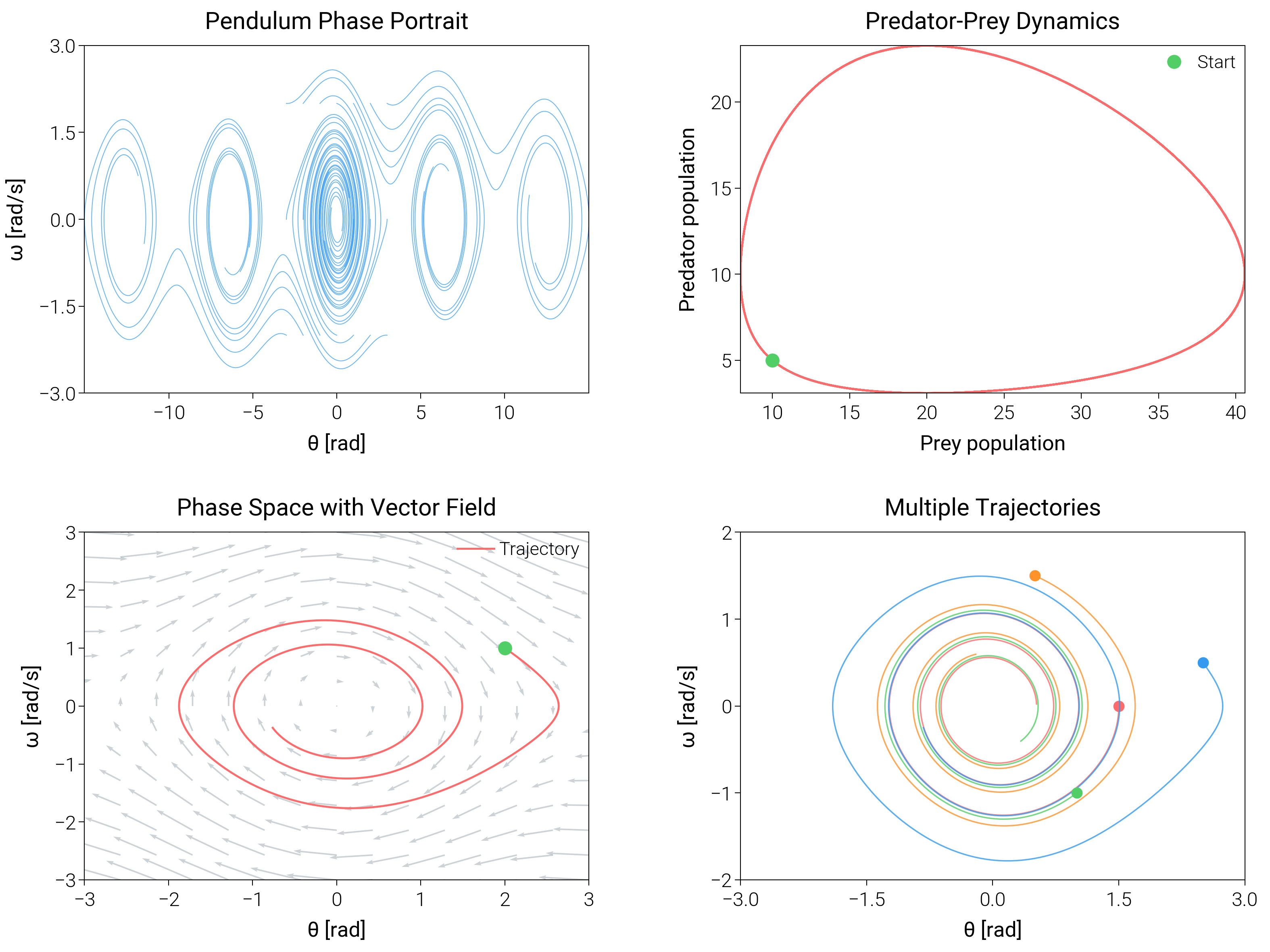
Phase Diagrams

Trace trajectories and vector fields to explain stability and cycles in dynamical systems.

import matplotlib.pyplot as plt
import numpy as np
from scipy.integrate import odeint

import dartwork_mpl as dm

# Apply scientific style preset
dm.style.use("scientific")


# Define dynamical systems
def pendulum(y, t, b, c):
    theta, omega = y
    dydt = [omega, -b * omega - c * np.sin(theta)]
    return dydt


def lotka_volterra(y, t, a, b, c, d):
    x, y_val = y
    dydt = [a * x - b * x * y_val, -c * y_val + d * x * y_val]
    return dydt


# Create figure
fig = plt.figure(figsize=(dm.cm2in(16), dm.cm2in(12)), dpi=300)

# Create GridSpec for 2x2 subplots
gs = fig.add_gridspec(
    nrows=2,
    ncols=2,
    left=0.08,
    right=0.98,
    top=0.95,
    bottom=0.08,
    wspace=0.3,
    hspace=0.4,
)

# Panel A: Simple pendulum phase portrait
ax1 = fig.add_subplot(gs[0, 0])
t = np.linspace(0, 20, 500)
for theta0 in [-3, -2, -1, 0, 1, 2, 3]:
    for omega0 in [-2, 0, 2]:
        y0 = [theta0, omega0]
        sol = odeint(pendulum, y0, t, args=(0.1, 1.0))
        ax1.plot(sol[:, 0], sol[:, 1], color="oc.blue5", lw=0.3, alpha=0.7)
ax1.set_xlabel("θ [rad]", fontsize=dm.fs(0))
ax1.set_ylabel("ω [rad/s]", fontsize=dm.fs(0))
ax1.set_title("Pendulum Phase Portrait", fontsize=dm.fs(1))
ax1.set_xticks([-10, -5, 0, 5, 10])
ax1.set_yticks([-3, -1.5, 0, 1.5, 3])

# Panel B: Predator-Prey (Lotka-Volterra)
ax2 = fig.add_subplot(gs[0, 1])
t_lv = np.linspace(0, 50, 1000)
y0_lv = [10, 5]
sol_lv = odeint(lotka_volterra, y0_lv, t_lv, args=(1.0, 0.1, 1.5, 0.075))
ax2.plot(sol_lv[:, 0], sol_lv[:, 1], color="oc.red5", lw=0.7)
ax2.plot(
    sol_lv[0, 0], sol_lv[0, 1], "o", color="oc.green5", ms=4, label="Start"
)
ax2.set_xlabel("Prey population", fontsize=dm.fs(0))
ax2.set_ylabel("Predator population", fontsize=dm.fs(0))
ax2.set_title("Predator-Prey Dynamics", fontsize=dm.fs(1))
ax2.legend(loc="best", fontsize=dm.fs(-1))

# Panel C: Vector field with trajectory
ax3 = fig.add_subplot(gs[1, 0])
# Create vector field
x_vec = np.linspace(-3, 3, 15)
y_vec = np.linspace(-3, 3, 15)
X, Y = np.meshgrid(x_vec, y_vec)
U = Y
V = -0.1 * Y - np.sin(X)
ax3.quiver(X, Y, U, V, alpha=0.6, width=0.003, scale=30, color="oc.gray5")
# Add trajectory
t_traj = np.linspace(0, 20, 500)
y0_traj = [2, 1]
sol_traj = odeint(pendulum, y0_traj, t_traj, args=(0.1, 1.0))
ax3.plot(
    sol_traj[:, 0], sol_traj[:, 1], color="oc.red5", lw=0.7, label="Trajectory"
)
ax3.plot(sol_traj[0, 0], sol_traj[0, 1], "o", color="oc.green5", ms=4)
ax3.set_xlabel("θ [rad]", fontsize=dm.fs(0))
ax3.set_ylabel("ω [rad/s]", fontsize=dm.fs(0))
ax3.set_title("Phase Space with Vector Field", fontsize=dm.fs(1))
ax3.legend(loc="best", fontsize=dm.fs(-1))
ax3.set_xlim(-3, 3)
ax3.set_ylim(-3, 3)

# Panel D: Multiple trajectories
ax4 = fig.add_subplot(gs[1, 1])
colors = ["oc.red5", "oc.blue5", "oc.green5", "oc.orange5"]
initial_conditions = [[1.5, 0], [2.5, 0.5], [1.0, -1], [0.5, 1.5]]
for ic, color in zip(initial_conditions, colors, strict=False):
    sol = odeint(pendulum, ic, t, args=(0.1, 1.0))
    ax4.plot(sol[:, 0], sol[:, 1], color=color, lw=0.5, alpha=0.8)
    ax4.plot(ic[0], ic[1], "o", color=color, ms=3)
ax4.set_xlabel("θ [rad]", fontsize=dm.fs(0))
ax4.set_ylabel("ω [rad/s]", fontsize=dm.fs(0))
ax4.set_title("Multiple Trajectories", fontsize=dm.fs(1))
ax4.set_xticks([-3, -1.5, 0, 1.5, 3])
ax4.set_yticks([-2, -1, 0, 1, 2])

# Optimize layout
dm.simple_layout(fig, gs=gs)

# Save and show plot
plt.show()