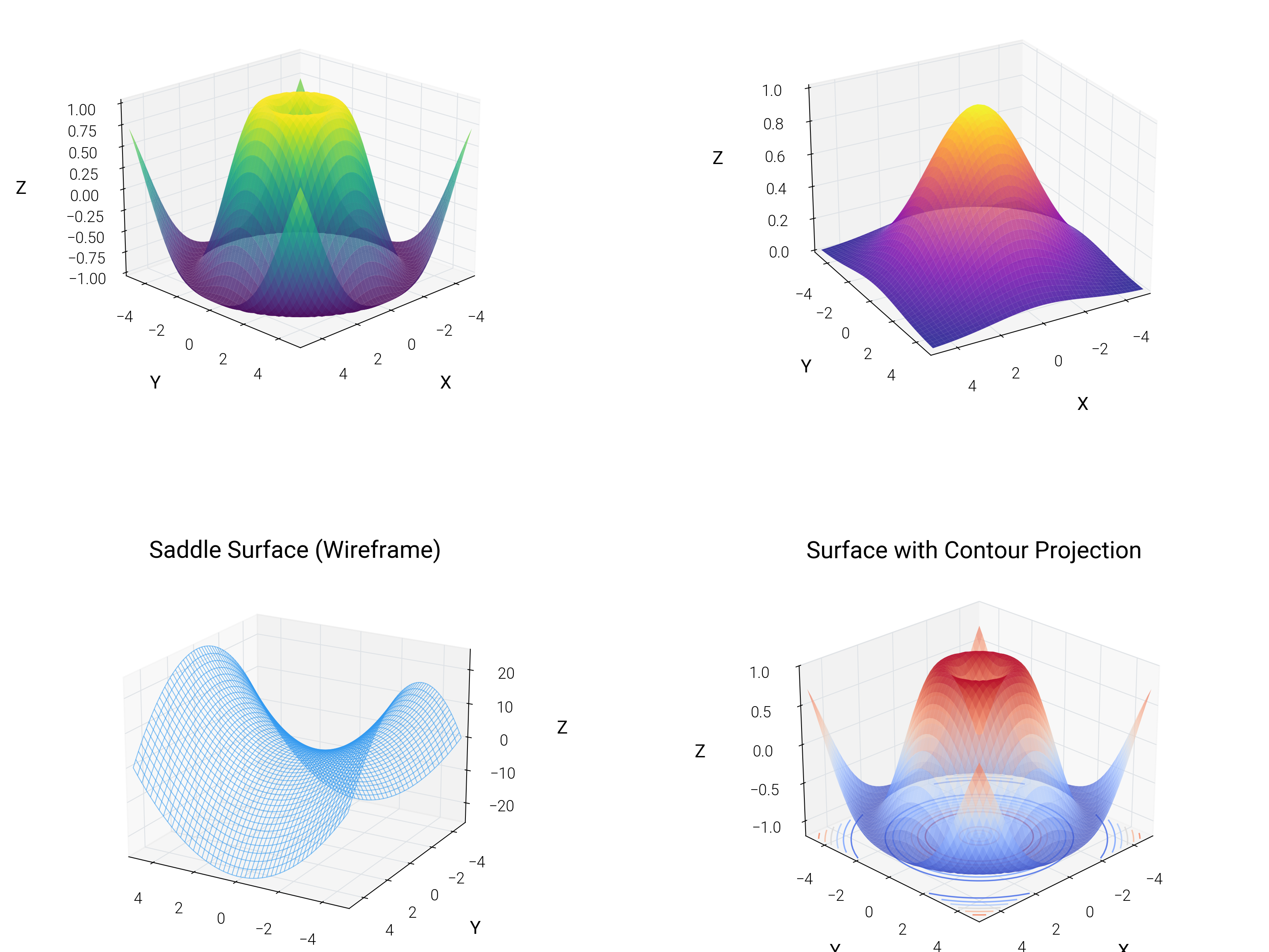
3D Surface Plots

Render smooth 3D surfaces with contours and lighting tweaks that photograph well in papers.

import matplotlib.pyplot as plt
import numpy as np

import dartwork_mpl as dm

# Apply scientific style preset
dm.style.use("scientific")

# Generate data
x = np.linspace(-5, 5, 50)
y = np.linspace(-5, 5, 50)
X, Y = np.meshgrid(x, y)
Z1 = np.sin(np.sqrt(X**2 + Y**2))
Z2 = np.exp(-(X**2 + Y**2) / 10)
Z3 = X**2 - Y**2

# Create figure
fig = plt.figure(figsize=(dm.cm2in(16), dm.cm2in(12)), dpi=300)

# Create GridSpec for 2x2 subplots
gs = fig.add_gridspec(
    nrows=2,
    ncols=2,
    left=0.02,
    right=0.98,
    top=0.95,
    bottom=0.05,
    wspace=0.15,
    hspace=0.45,
)

# Panel A: Surface plot
ax1 = fig.add_subplot(gs[0, 0], projection="3d")
surf1 = ax1.plot_surface(
    X, Y, Z1, cmap="viridis", alpha=0.8, linewidth=0, antialiased=True
)
ax1.set_xlabel("X", fontsize=dm.fs(-1), labelpad=0)
ax1.set_ylabel("Y", fontsize=dm.fs(-1), labelpad=0)
ax1.set_zlabel("Z", fontsize=dm.fs(-1), labelpad=0)
ax1.set_title("Sine Wave Surface", fontsize=dm.fs(1), pad=2)
ax1.tick_params(labelsize=dm.fs(-2), pad=0)
ax1.view_init(elev=20, azim=45)

# Panel B: Gaussian surface
ax2 = fig.add_subplot(gs[0, 1], projection="3d")
surf2 = ax2.plot_surface(
    X, Y, Z2, cmap="plasma", alpha=0.8, linewidth=0, antialiased=True
)
ax2.set_xlabel("X", fontsize=dm.fs(-1), labelpad=0)
ax2.set_ylabel("Y", fontsize=dm.fs(-1), labelpad=0)
ax2.set_zlabel("Z", fontsize=dm.fs(-1), labelpad=0)
ax2.set_title("Gaussian Surface", fontsize=dm.fs(1), pad=2)
ax2.tick_params(labelsize=dm.fs(-2), pad=0)
ax2.view_init(elev=25, azim=60)

# Panel C: Wireframe
ax3 = fig.add_subplot(gs[1, 0], projection="3d")
ax3.plot_wireframe(X, Y, Z3, color="oc.blue5", alpha=0.6, linewidth=0.3)
ax3.set_xlabel("X", fontsize=dm.fs(-1), labelpad=0)
ax3.set_ylabel("Y", fontsize=dm.fs(-1), labelpad=0)
ax3.set_zlabel("Z", fontsize=dm.fs(-1), labelpad=0)
ax3.set_title("Saddle Surface (Wireframe)", fontsize=dm.fs(1), pad=2)
ax3.tick_params(labelsize=dm.fs(-2), pad=0)
ax3.view_init(elev=20, azim=120)

# Panel D: Contour3D projection
ax4 = fig.add_subplot(gs[1, 1], projection="3d")
# Surface with contour projection
surf4 = ax4.plot_surface(
    X, Y, Z1, cmap="coolwarm", alpha=0.7, linewidth=0, antialiased=True
)
# Project contours on bottom
ax4.contour(X, Y, Z1, zdir="z", offset=-1.2, cmap="coolwarm", linewidths=0.5)
ax4.set_xlabel("X", fontsize=dm.fs(-1), labelpad=0)
ax4.set_ylabel("Y", fontsize=dm.fs(-1), labelpad=0)
ax4.set_zlabel("Z", fontsize=dm.fs(-1), labelpad=0)
ax4.set_title("Surface with Contour Projection", fontsize=dm.fs(1), pad=2)
ax4.set_zlim(-1.2, 1)
ax4.tick_params(labelsize=dm.fs(-2), pad=0)
ax4.view_init(elev=25, azim=45)

# Optimize layout
dm.simple_layout(fig, gs=gs)

# Save and show plot
plt.show()