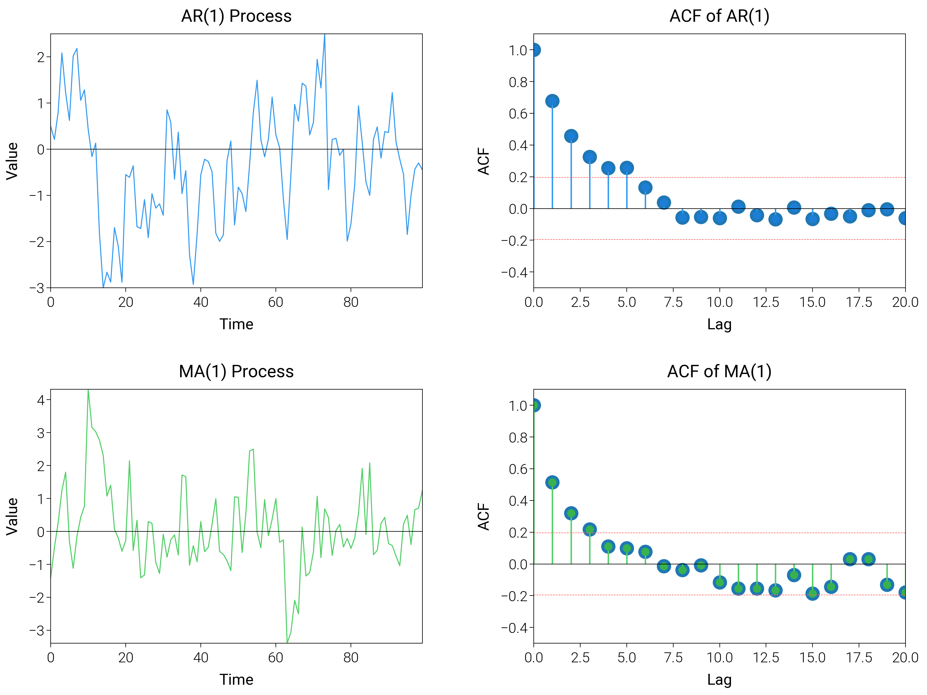
Autocorrelation Analysis

Plot ACF and PACF with significance bounds to quickly judge lag structure.

import matplotlib.pyplot as plt
import numpy as np

import dartwork_mpl as dm

dm.style.use("scientific")

# Generate time series
np.random.seed(42)
n = 100
# AR(1) process
phi = 0.7
ar1 = np.zeros(n)
ar1[0] = np.random.randn()
for i in range(1, n):
    ar1[i] = phi * ar1[i - 1] + np.random.randn()

# MA(1) process
theta = 0.6
ma1 = np.random.randn(n)
for i in range(1, n):
    ma1[i] = np.random.randn() + theta * ma1[i - 1]


# Calculate ACF
def acf(x, lags):
    return np.array(
        [1] + [np.corrcoef(x[:-i], x[i:])[0, 1] for i in range(1, lags + 1)]
    )


lags = 20
acf_ar = acf(ar1, lags)
acf_ma = acf(ma1, lags)

fig = plt.figure(figsize=(dm.cm2in(16), dm.cm2in(12)), dpi=300)
gs = fig.add_gridspec(
    nrows=2,
    ncols=2,
    left=0.08,
    right=0.98,
    top=0.95,
    bottom=0.08,
    wspace=0.3,
    hspace=0.4,
)

# Panel A: AR(1) time series
ax1 = fig.add_subplot(gs[0, 0])
ax1.plot(ar1, color="oc.blue5", lw=0.5)
ax1.set_xlabel("Time", fontsize=dm.fs(0))
ax1.set_ylabel("Value", fontsize=dm.fs(0))
ax1.set_title("AR(1) Process", fontsize=dm.fs(1))
ax1.axhline(y=0, color="k", lw=0.3)

# Panel B: ACF of AR(1)
ax2 = fig.add_subplot(gs[0, 1])
ax2.stem(range(lags + 1), acf_ar, basefmt=" ")
markerline, stemlines, baseline = ax2.stem(range(lags + 1), acf_ar, basefmt=" ")
plt.setp(stemlines, "color", "oc.blue5", "linewidth", 0.7)
plt.setp(markerline, "color", "oc.blue7", "markersize", 3)
ax2.axhline(y=0, color="k", lw=0.3)
ax2.axhline(y=1.96 / np.sqrt(n), color="oc.red5", lw=0.3, linestyle="--")
ax2.axhline(y=-1.96 / np.sqrt(n), color="oc.red5", lw=0.3, linestyle="--")
ax2.set_xlabel("Lag", fontsize=dm.fs(0))
ax2.set_ylabel("ACF", fontsize=dm.fs(0))
ax2.set_title("ACF of AR(1)", fontsize=dm.fs(1))
ax2.set_ylim(-0.5, 1.1)

# Panel C: MA(1) time series
ax3 = fig.add_subplot(gs[1, 0])
ax3.plot(ma1, color="oc.green5", lw=0.5)
ax3.set_xlabel("Time", fontsize=dm.fs(0))
ax3.set_ylabel("Value", fontsize=dm.fs(0))
ax3.set_title("MA(1) Process", fontsize=dm.fs(1))
ax3.axhline(y=0, color="k", lw=0.3)

# Panel D: ACF of MA(1)
ax4 = fig.add_subplot(gs[1, 1])
ax4.stem(range(lags + 1), acf_ma, basefmt=" ")
markerline2, stemlines2, baseline2 = ax4.stem(
    range(lags + 1), acf_ma, basefmt=" "
)
plt.setp(stemlines2, "color", "oc.green5", "linewidth", 0.7)
plt.setp(markerline2, "color", "oc.green7", "markersize", 3)
ax4.axhline(y=0, color="k", lw=0.3)
ax4.axhline(y=1.96 / np.sqrt(n), color="oc.red5", lw=0.3, linestyle="--")
ax4.axhline(y=-1.96 / np.sqrt(n), color="oc.red5", lw=0.3, linestyle="--")
ax4.set_xlabel("Lag", fontsize=dm.fs(0))
ax4.set_ylabel("ACF", fontsize=dm.fs(0))
ax4.set_title("ACF of MA(1)", fontsize=dm.fs(1))
ax4.set_ylim(-0.5, 1.1)

dm.simple_layout(fig, gs=gs)
plt.show()