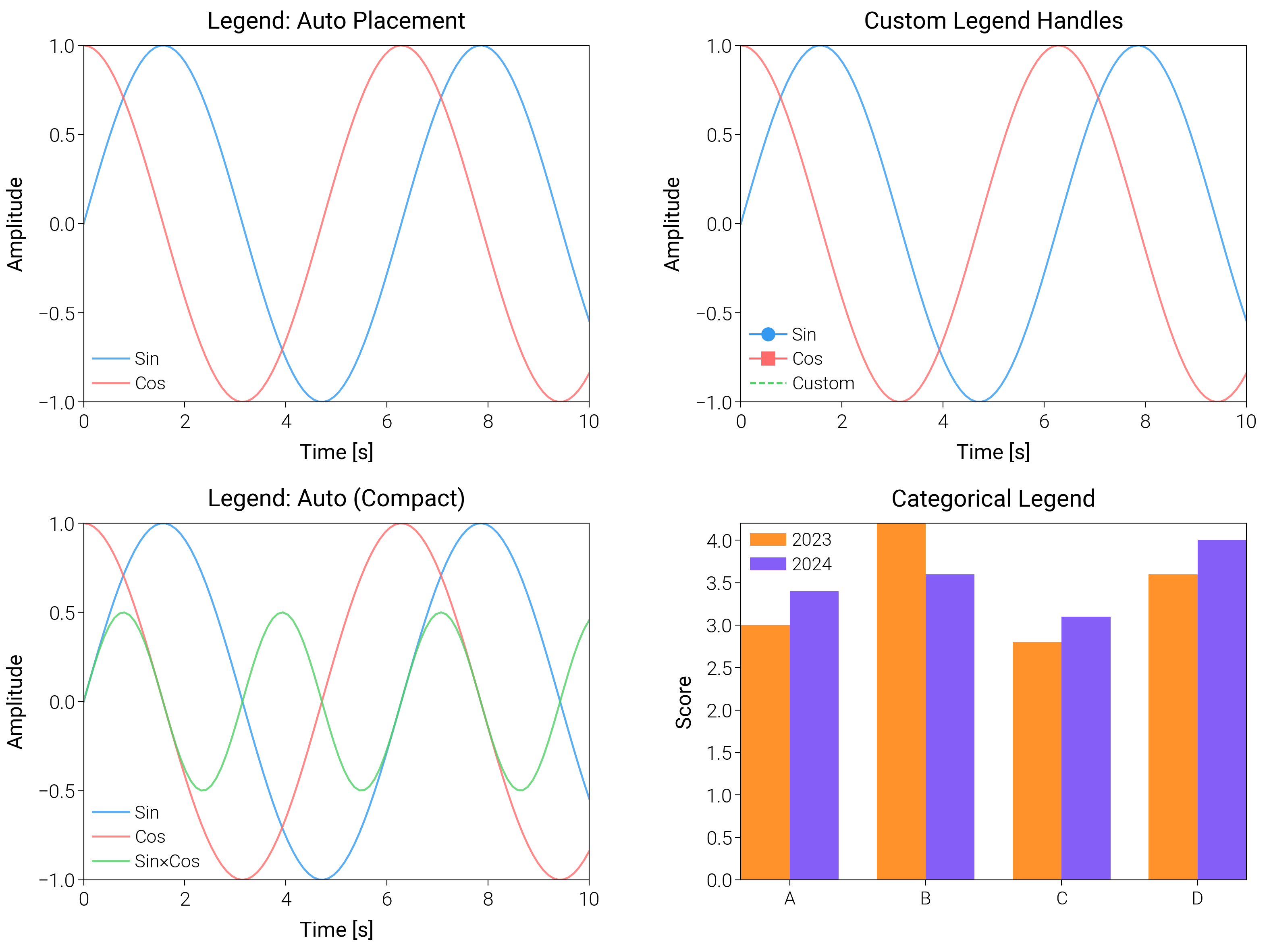
Legends

Design legends with columns, geoms, backgrounds, and aligned handles that match publication styles.

import matplotlib.pyplot as plt
import numpy as np

import dartwork_mpl as dm

# Apply scientific style preset
# Default: font.size=7.5, lines.linewidth=0.5, axes.linewidth=0.3
dm.style.use("scientific")

# Generate sample data
x = np.linspace(0, 10, 100)
y1 = np.sin(x)
y2 = np.cos(x)
y3 = np.sin(x) * np.cos(x)

# Create figure
# Two-by-two layout
fig = plt.figure(figsize=(dm.cm2in(16), dm.cm2in(12)), dpi=300)

# Create GridSpec for 4 subplots
gs = fig.add_gridspec(
    nrows=2,
    ncols=2,
    left=0.08,
    right=0.98,
    top=0.92,
    bottom=0.12,
    wspace=0.3,
    hspace=0.34,
)

# Panel A: Multiple legend locations
ax1 = fig.add_subplot(gs[0, 0])
ax1.plot(x, y1, color="oc.blue5", lw=0.7, label="Sin", alpha=0.8)
ax1.plot(x, y2, color="oc.red5", lw=0.7, label="Cos", alpha=0.8)
# Legend: loc='best', fontsize=dm.fs(-1), ncol=1
ax1.legend(loc="best", fontsize=dm.fs(-1), ncol=1, framealpha=0.9)
ax1.set_xlabel("Time [s]", fontsize=dm.fs(0))
ax1.set_ylabel("Amplitude", fontsize=dm.fs(0))
ax1.set_title("Legend: Auto Placement", fontsize=dm.fs(1))
ax1.set_xticks([0, 2, 4, 6, 8, 10])
ax1.set_yticks([-1, -0.5, 0, 0.5, 1])

# Panel B: Custom legend handles
ax2 = fig.add_subplot(gs[0, 1])
(line1,) = ax2.plot(x, y1, color="oc.blue5", lw=0.7, alpha=0.8)
(line2,) = ax2.plot(x, y2, color="oc.red5", lw=0.7, alpha=0.8)
# Create custom handles: explicit marker and line styles
from matplotlib.lines import Line2D

custom_handles = [
    Line2D(
        [0],
        [0],
        color="oc.blue5",
        lw=0.7,
        marker="o",
        markersize=4,
        label="Sin",
    ),
    Line2D(
        [0], [0], color="oc.red5", lw=0.7, marker="s", markersize=4, label="Cos"
    ),
    Line2D([0], [0], color="oc.green5", lw=0.7, linestyle="--", label="Custom"),
]
ax2.legend(
    handles=custom_handles,
    loc="best",
    fontsize=dm.fs(-1),
    ncol=1,
    framealpha=0.9,
)
ax2.set_xlabel("Time [s]", fontsize=dm.fs(0))
ax2.set_ylabel("Amplitude", fontsize=dm.fs(0))
ax2.set_title("Custom Legend Handles", fontsize=dm.fs(1))
ax2.set_xticks([0, 2, 4, 6, 8, 10])
ax2.set_yticks([-1, -0.5, 0, 0.5, 1])

# Panel C: Legend inside axes (kept compact for thumbnails)
ax3 = fig.add_subplot(gs[1, 0])
ax3.plot(x, y1, color="oc.blue5", lw=0.7, label="Sin", alpha=0.8)
ax3.plot(x, y2, color="oc.red5", lw=0.7, label="Cos", alpha=0.8)
ax3.plot(x, y3, color="oc.green5", lw=0.7, label="Sin×Cos", alpha=0.8)
# Legend tucked inside to avoid overflow
ax3.legend(loc="best", fontsize=dm.fs(-1), ncol=1, framealpha=0.9)
ax3.set_xlabel("Time [s]", fontsize=dm.fs(0))
ax3.set_ylabel("Amplitude", fontsize=dm.fs(0))
ax3.set_title("Legend: Auto (Compact)", fontsize=dm.fs(1))
ax3.set_xticks([0, 2, 4, 6, 8, 10])
ax3.set_yticks([-1, -0.5, 0, 0.5, 1])

# Panel D: Patch legend for categorical bars
ax4 = fig.add_subplot(gs[1, 1])
cats = ["A", "B", "C", "D"]
idx = np.arange(len(cats))
bar1 = ax4.bar(
    idx - 0.18, [3, 4.2, 2.8, 3.6], width=0.36, color="oc.orange5", label="2023"
)
bar2 = ax4.bar(
    idx + 0.18,
    [3.4, 3.6, 3.1, 4.0],
    width=0.36,
    color="oc.violet5",
    label="2024",
)
ax4.set_xticks(idx)
ax4.set_xticklabels(cats, fontsize=dm.fs(-1))
ax4.set_ylabel("Score", fontsize=dm.fs(0))
ax4.set_title("Categorical Legend", fontsize=dm.fs(1))
ax4.legend(loc="best", fontsize=dm.fs(-1), framealpha=0.9)

# Optimize layout
dm.simple_layout(fig, gs=gs)

# Show plot
plt.show()