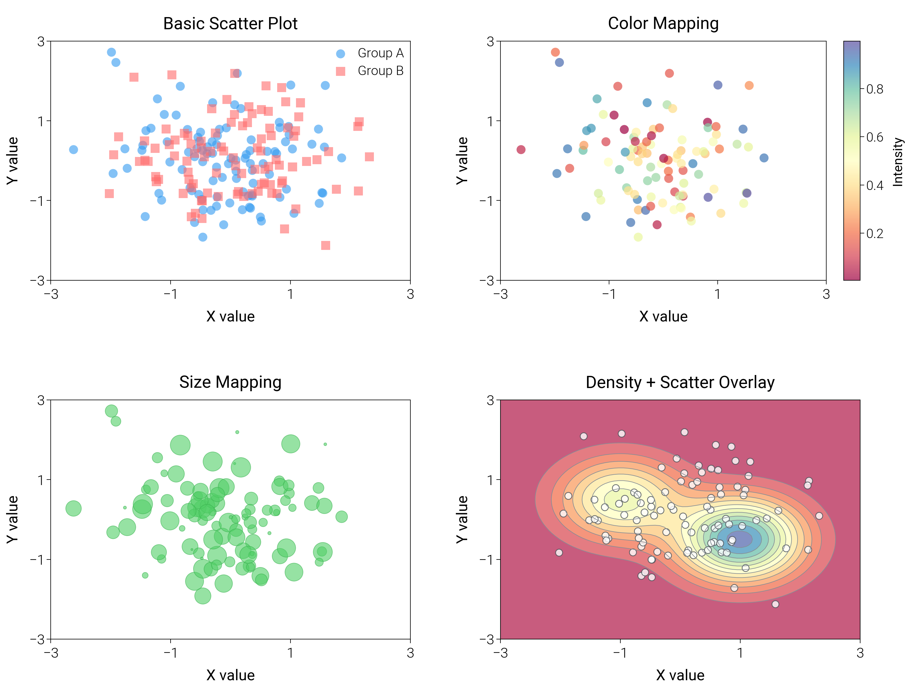
Scatter Plots

Contrast marker shapes, color encodings, and density shading to show clusters and overlaps more clearly.

import matplotlib.pyplot as plt
import numpy as np
from mpl_toolkits.axes_grid1 import make_axes_locatable

import dartwork_mpl as dm

# Apply scientific style preset
# Default: font.size=7.5, lines.linewidth=0.5, axes.linewidth=0.3
dm.style.use("scientific")

# Generate sample data
np.random.seed(42)
n = 100
x1 = np.random.randn(n)
y1 = np.random.randn(n)
x2 = np.random.randn(n)
y2 = np.random.randn(n)
x3 = np.random.randn(n)
y3 = np.random.randn(n)

# Color mapping data
colors = np.random.rand(n)
# Size mapping data
sizes = 100 * np.random.rand(n)

# Create figure
# Square-ish layout: 16 cm wide, 12 cm tall, 2x2 grid
fig = plt.figure(figsize=(dm.cm2in(16), dm.cm2in(12)), dpi=300)

# Create GridSpec for 4 subplots (2x2)
gs = fig.add_gridspec(
    nrows=2,
    ncols=2,
    left=0.08,
    right=0.98,
    top=0.92,
    bottom=0.12,
    wspace=0.25,
    hspace=0.5,
)

# Panel A: Basic scatter with different markers
ax1 = fig.add_subplot(gs[0, 0])
# Explicit parameters: markersize=4, lw=0 (no edge), alpha=0.6
ax1.scatter(
    x1,
    y1,
    c="oc.blue5",
    s=20,
    marker="o",
    edgecolors="none",
    alpha=0.6,
    label="Group A",
)
ax1.scatter(
    x2,
    y2,
    c="oc.red5",
    s=20,
    marker="s",
    edgecolors="none",
    alpha=0.6,
    label="Group B",
)
ax1.set_xlabel("X value", fontsize=dm.fs(0))
ax1.set_ylabel("Y value", fontsize=dm.fs(0))
ax1.set_title("Basic Scatter Plot", fontsize=dm.fs(1))
ax1.legend(loc="best", fontsize=dm.fs(-1), ncol=1)
# Set explicit ticks
ax1.set_xticks([-3, -1, 1, 3])
ax1.set_yticks([-3, -1, 1, 3])
ax1.set_xlim(-3, 3)
ax1.set_ylim(-3, 3)

# Panel B: Scatter with color mapping
ax2 = fig.add_subplot(gs[0, 1])
# Color mapping: c=colors, cmap='dm.Spectral', s=20 (size), alpha=0.7
scatter2 = ax2.scatter(
    x1, y1, c=colors, s=20, cmap="dm.Spectral", edgecolors="none", alpha=0.7
)
ax2.set_xlabel("X value", fontsize=dm.fs(0))
ax2.set_ylabel("Y value", fontsize=dm.fs(0))
ax2.set_title("Color Mapping", fontsize=dm.fs(1))
# Add colorbar with dedicated side axis
divider = make_axes_locatable(ax2)
cax2 = divider.append_axes("right", size="5%", pad=0.12)
cbar2 = fig.colorbar(scatter2, cax=cax2)
cbar2.set_label("Intensity", fontsize=dm.fs(-1))
cbar2.ax.tick_params(labelsize=dm.fs(-1))
# Set explicit ticks/limits
ax2.set_xticks([-3, -1, 1, 3])
ax2.set_yticks([-3, -1, 1, 3])
ax2.set_xlim(-3, 3)
ax2.set_ylim(-3, 3)

# Panel C: Scatter with size mapping
ax3 = fig.add_subplot(gs[1, 0])
# Size mapping: s=sizes, c='oc.green5', alpha=0.6
scatter3 = ax3.scatter(
    x1,
    y1,
    s=sizes,
    c="oc.green5",
    edgecolors="oc.green7",
    linewidths=0.3,
    alpha=0.6,
)
ax3.set_xlabel("X value", fontsize=dm.fs(0))
ax3.set_ylabel("Y value", fontsize=dm.fs(0))
ax3.set_title("Size Mapping", fontsize=dm.fs(1))
# Set explicit ticks
ax3.set_xticks([-3, -1, 1, 3])
ax3.set_yticks([-3, -1, 1, 3])
ax3.set_xlim(-3, 3)
ax3.set_ylim(-3, 3)

# Panel D: Density background + contour overlays
ax4 = fig.add_subplot(gs[1, 1])
grid_x, grid_y = np.meshgrid(np.linspace(-3, 3, 80), np.linspace(-3, 3, 80))
dens = np.exp(-((grid_x - 1) ** 2 + (grid_y + 0.5) ** 2)) + 0.6 * np.exp(
    -((grid_x + 1) ** 2 + (grid_y - 0.5) ** 2)
)
ax4.contourf(grid_x, grid_y, dens, cmap="dm.Spectral", alpha=0.7, levels=12)
ax4.contour(grid_x, grid_y, dens, colors="oc.gray6", linewidths=0.3, levels=12)
ax4.scatter(
    x2, y2, c="white", s=12, edgecolors="oc.gray7", linewidths=0.4, alpha=0.8
)
ax4.set_xlabel("X value", fontsize=dm.fs(0))
ax4.set_ylabel("Y value", fontsize=dm.fs(0))
ax4.set_title("Density + Scatter Overlay", fontsize=dm.fs(1))
ax4.set_xticks([-3, -1, 1, 3])
ax4.set_yticks([-3, -1, 1, 3])
ax4.set_xlim(-3, 3)
ax4.set_ylim(-3, 3)

# Optimize layout
dm.simple_layout(fig, gs=gs)

# Show plot
plt.show()