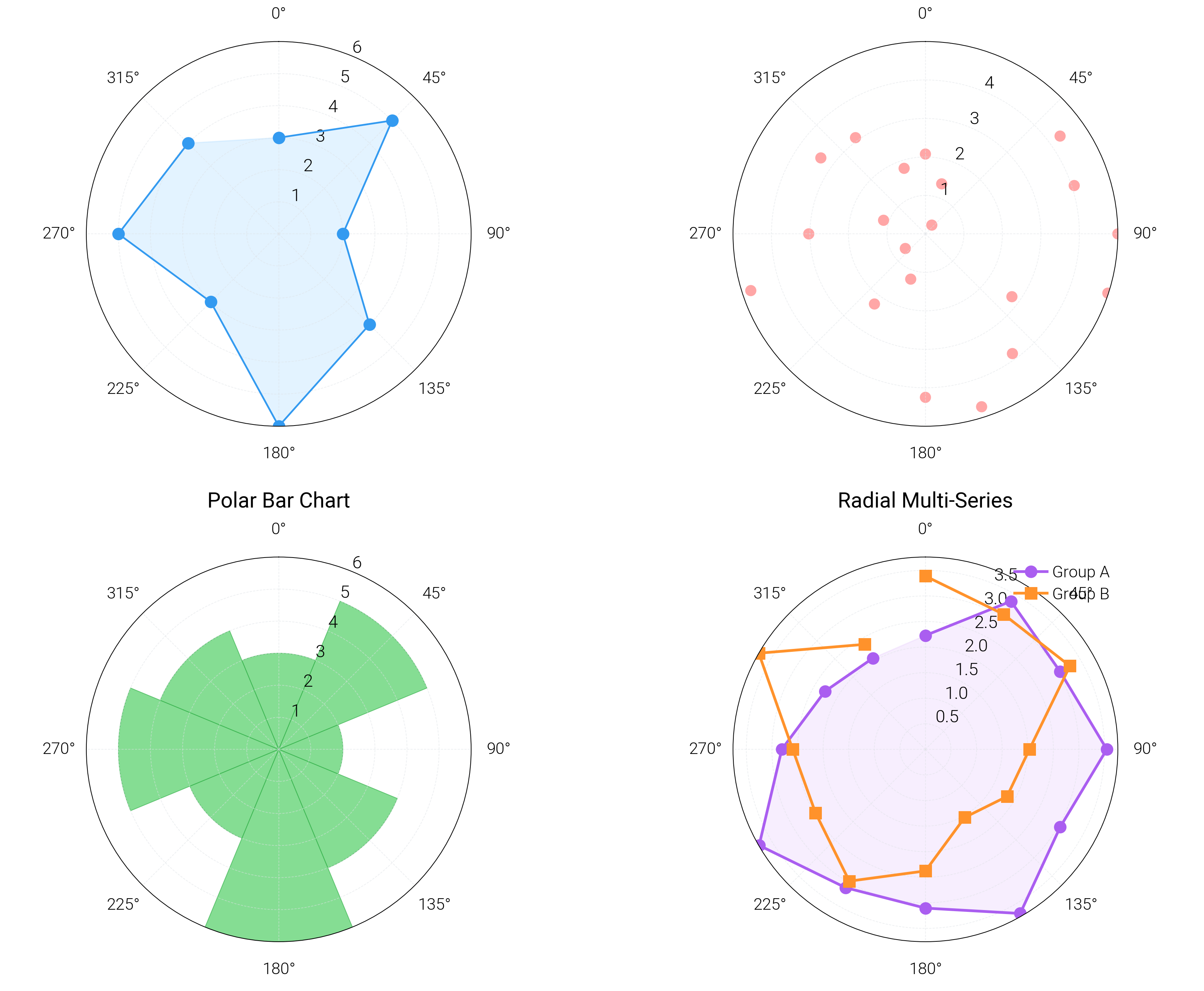
Polar Plots

Create polar lines, scatters, and radial bars tuned for angle grids and clear radial labels.

import matplotlib.pyplot as plt
import numpy as np

import dartwork_mpl as dm

# Apply scientific style preset
# Default: font.size=7.5, lines.linewidth=0.5, axes.linewidth=0.3
dm.style.use("scientific")

# Generate sample data
theta = np.linspace(0, 2 * np.pi, 8, endpoint=False)
r1 = np.array([3, 5, 2, 4, 6, 3, 5, 4])
r2 = np.random.rand(20) * 5
theta2 = np.linspace(0, 2 * np.pi, 20, endpoint=False)

# Create figure (roomier to avoid clipped titles): ~17 cm wide, 14 cm tall
fig = plt.figure(figsize=(dm.cm2in(17), dm.cm2in(14)), dpi=300)

# Create GridSpec for 4 subplots with polar projection (2x2)
gs = fig.add_gridspec(
    nrows=2,
    ncols=2,
    left=0.07,
    right=0.95,
    top=0.96,
    bottom=0.08,
    wspace=0.16,
    hspace=0.34,
)

theta_labels_deg = np.arange(0, 360, 45)


def apply_theta_labels(ax, frac=1.04, pad=2):
    """Place all theta tick labels at a consistent distance from the rim."""
    ax.set_thetagrids(theta_labels_deg)
    ax.tick_params(axis="x", labelsize=dm.fs(-1), pad=pad)


# Panel A: Basic polar plot
ax1 = fig.add_subplot(gs[0, 0], projection="polar")
# Explicit parameters: lw=0.7, marker='o', markersize=4
ax1.plot(
    theta, r1, color="oc.blue5", lw=0.7, marker="o", markersize=4, label="Data"
)
ax1.fill(theta, r1, color="oc.blue2", alpha=0.3)
ax1.set_title("Basic Polar Plot", fontsize=dm.fs(1), pad=20)
ax1.set_theta_zero_location("N")
ax1.set_theta_direction(-1)
ax1.grid(True, linestyle="--", linewidth=0.3, alpha=0.5)
apply_theta_labels(ax1)

# Panel B: Polar scatter plot
ax2 = fig.add_subplot(gs[0, 1], projection="polar")
# Explicit parameters: s=20, alpha=0.6
ax2.scatter(theta2, r2, c="oc.red5", s=20, alpha=0.6, edgecolors="none")
ax2.set_title("Polar Scatter Plot", fontsize=dm.fs(1), pad=20)
ax2.set_theta_zero_location("N")
ax2.set_theta_direction(-1)
ax2.grid(True, linestyle="--", linewidth=0.3, alpha=0.5)
apply_theta_labels(ax2)

# Panel C: Polar bar chart
ax3 = fig.add_subplot(gs[1, 0], projection="polar")
# Explicit parameters: width=0.5, alpha=0.7, edgecolor, linewidth=0.3
width = 2 * np.pi / len(theta)
bars = ax3.bar(
    theta,
    r1,
    width=width,
    color="oc.green5",
    alpha=0.7,
    edgecolor="oc.green7",
    linewidth=0.3,
)
ax3.set_title("Polar Bar Chart", fontsize=dm.fs(1), pad=20)
ax3.set_theta_zero_location("N")
ax3.set_theta_direction(-1)
ax3.grid(True, linestyle="--", linewidth=0.3, alpha=0.5)
apply_theta_labels(ax3)

# Panel D: Multi-group radial comparison
ax4 = fig.add_subplot(gs[1, 1], projection="polar")
theta_groups = np.linspace(0, 2 * np.pi, 12, endpoint=False)
group_a = 2 + np.random.rand(len(theta_groups)) * 2
group_b = 1.5 + np.random.rand(len(theta_groups)) * 2.5
ax4.plot(
    theta_groups,
    group_a,
    color="oc.purple5",
    lw=1.1,
    marker="o",
    markersize=4,
    label="Group A",
)
ax4.plot(
    theta_groups,
    group_b,
    color="oc.orange5",
    lw=1.1,
    marker="s",
    markersize=4,
    label="Group B",
)
ax4.fill(theta_groups, group_a, color="oc.purple2", alpha=0.25)
ax4.set_title("Radial Multi-Series", fontsize=dm.fs(1), pad=20)
ax4.legend(loc="best", fontsize=dm.fs(-1))
ax4.set_theta_zero_location("N")
ax4.set_theta_direction(-1)
ax4.grid(True, linestyle="--", linewidth=0.3, alpha=0.5)
apply_theta_labels(ax4)

# Optimize layout
dm.simple_layout(fig, gs=gs)

# Show plot
plt.show()