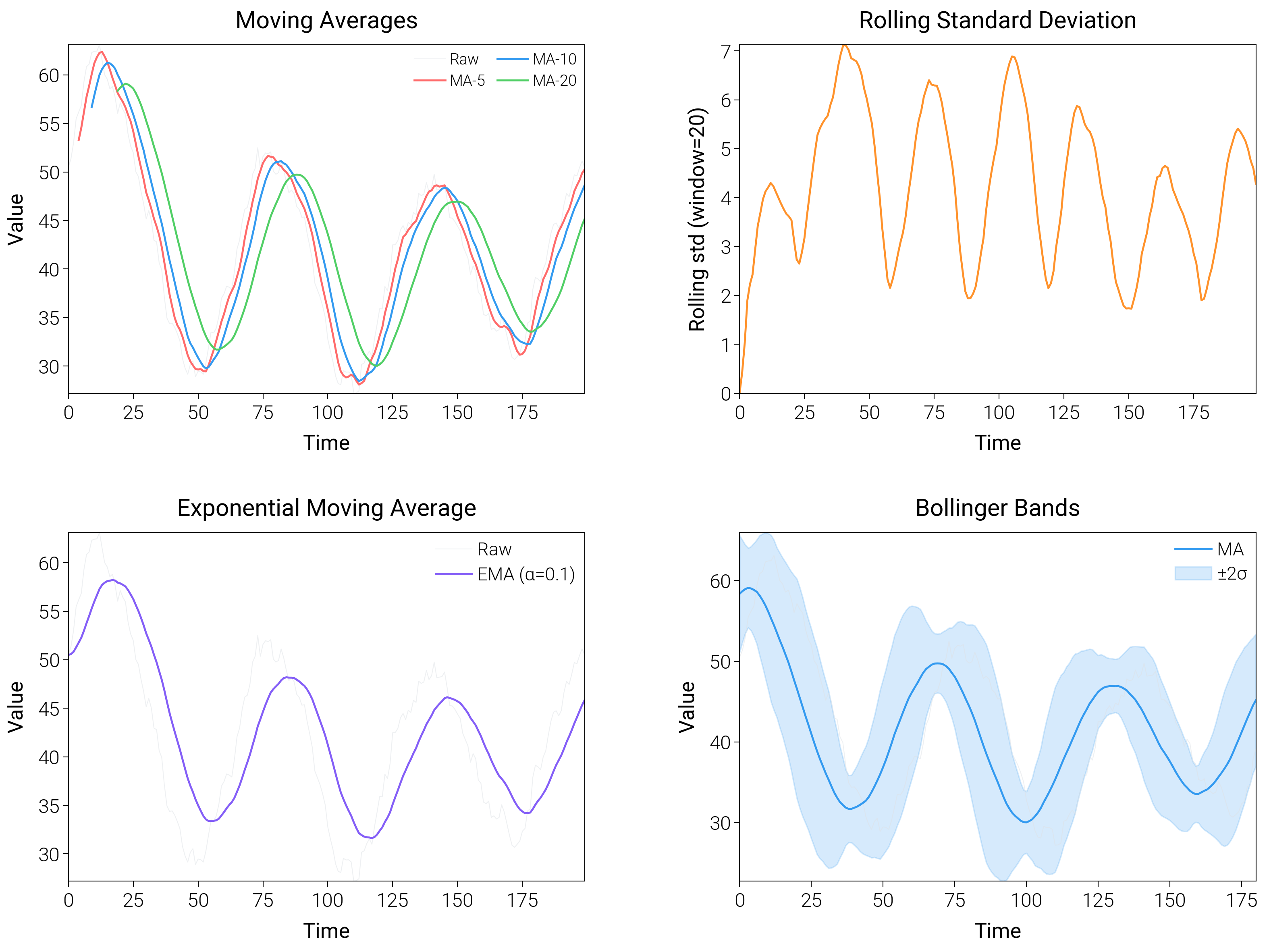
Rolling Statistics

Track rolling means and variances with window markers to show stability and volatility over time.

import matplotlib.pyplot as plt
import numpy as np

import dartwork_mpl as dm

dm.style.use("scientific")

# Generate data
np.random.seed(42)
n = 200
t = np.arange(n)
data = 50 + np.cumsum(np.random.randn(n)) + 10 * np.sin(t / 10)

# Calculate rolling statistics
window_sizes = [5, 10, 20]
rolling_means = [
    np.convolve(data, np.ones(w) / w, mode="valid") for w in window_sizes
]

fig = plt.figure(figsize=(dm.cm2in(16), dm.cm2in(12)), dpi=300)
gs = fig.add_gridspec(
    nrows=2,
    ncols=2,
    left=0.08,
    right=0.98,
    top=0.95,
    bottom=0.08,
    wspace=0.3,
    hspace=0.4,
)

# Panel A: Raw data with moving averages
ax1 = fig.add_subplot(gs[0, 0])
ax1.plot(t, data, color="oc.gray3", lw=0.3, alpha=0.5, label="Raw")
colors = ["oc.red5", "oc.blue5", "oc.green5"]
for _, (rm, w, c) in enumerate(
    zip(rolling_means, window_sizes, colors, strict=False)
):
    ax1.plot(t[w - 1 :], rm, color=c, lw=0.7, label=f"MA-{w}")
ax1.set_xlabel("Time", fontsize=dm.fs(0))
ax1.set_ylabel("Value", fontsize=dm.fs(0))
ax1.set_title("Moving Averages", fontsize=dm.fs(1))
ax1.legend(loc="best", fontsize=dm.fs(-2), ncol=2)

# Panel B: Rolling standard deviation
ax2 = fig.add_subplot(gs[0, 1])
rolling_std = np.array(
    [np.std(data[max(0, i - 20) : i + 1]) for i in range(len(data))]
)
ax2.plot(t, rolling_std, color="oc.orange5", lw=0.7)
ax2.set_xlabel("Time", fontsize=dm.fs(0))
ax2.set_ylabel("Rolling std (window=20)", fontsize=dm.fs(0))
ax2.set_title("Rolling Standard Deviation", fontsize=dm.fs(1))

# Panel C: Exponential moving average
ax3 = fig.add_subplot(gs[1, 0])
alpha = 0.1
ema = np.zeros(n)
ema[0] = data[0]
for i in range(1, n):
    ema[i] = alpha * data[i] + (1 - alpha) * ema[i - 1]
ax3.plot(t, data, color="oc.gray3", lw=0.3, alpha=0.5, label="Raw")
ax3.plot(t, ema, color="oc.violet5", lw=0.7, label=f"EMA (α={alpha})")
ax3.set_xlabel("Time", fontsize=dm.fs(0))
ax3.set_ylabel("Value", fontsize=dm.fs(0))
ax3.set_title("Exponential Moving Average", fontsize=dm.fs(1))
ax3.legend(loc="best", fontsize=dm.fs(-1))

# Panel D: Bollinger bands
ax4 = fig.add_subplot(gs[1, 1])
ma = np.convolve(data, np.ones(20) / 20, mode="valid")
std = np.array([np.std(data[i : i + 20]) for i in range(len(data) - 19)])
upper = ma + 2 * std
lower = ma - 2 * std
ax4.plot(t[: len(ma)], data[: len(ma)], color="oc.gray3", lw=0.3, alpha=0.5)
ax4.plot(t[: len(ma)], ma, color="oc.blue5", lw=0.7, label="MA")
ax4.fill_between(
    t[: len(ma)], lower, upper, color="oc.blue5", alpha=0.2, label="±2σ"
)
ax4.set_xlabel("Time", fontsize=dm.fs(0))
ax4.set_ylabel("Value", fontsize=dm.fs(0))
ax4.set_title("Bollinger Bands", fontsize=dm.fs(1))
ax4.legend(loc="best", fontsize=dm.fs(-1))

dm.simple_layout(fig, gs=gs)
plt.show()