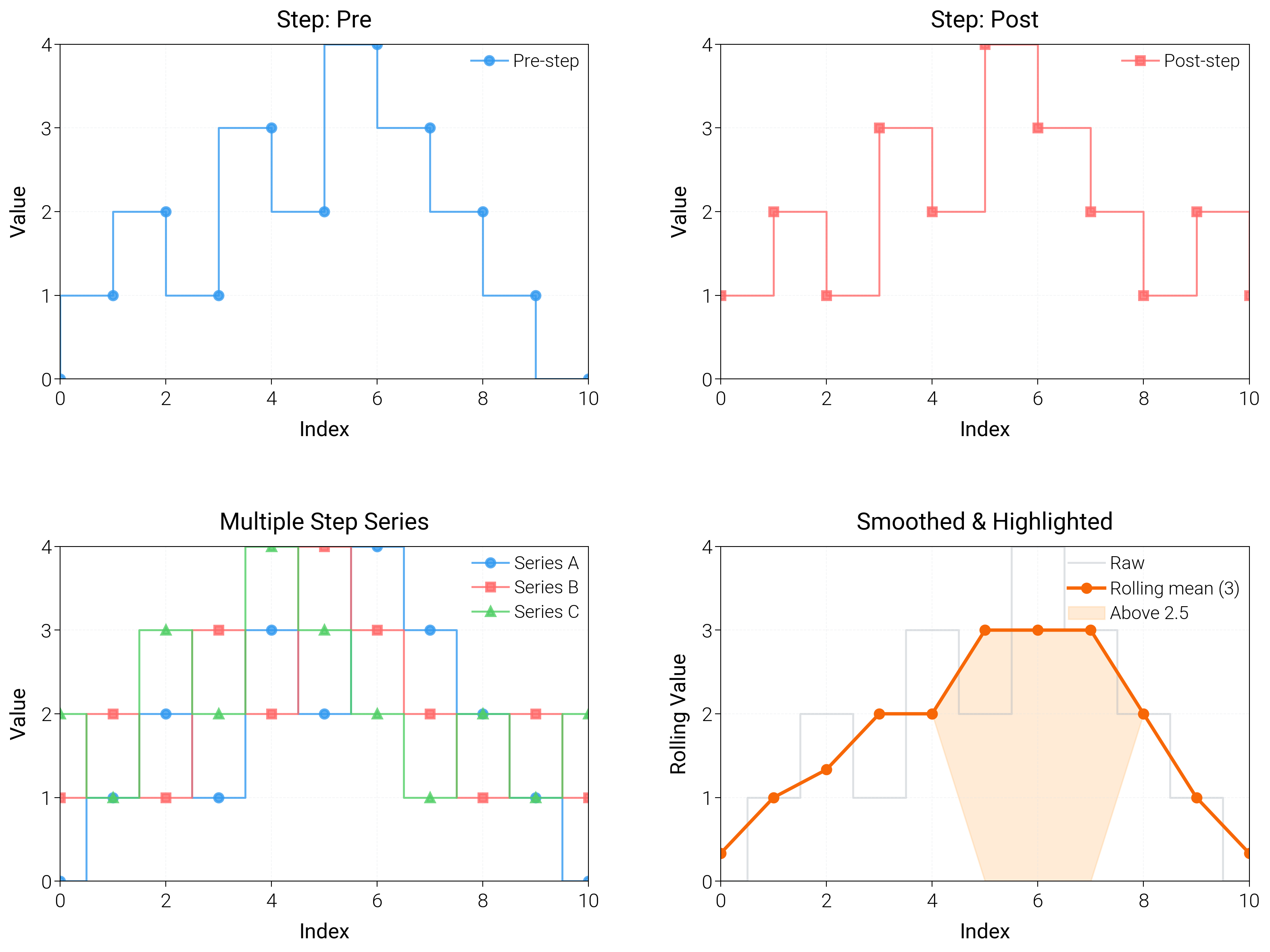
Step Plots

Build step charts that expose change points, holding periods, and cumulative shifts.

import matplotlib.pyplot as plt
import numpy as np

import dartwork_mpl as dm

# Apply scientific style preset
# Default: font.size=7.5, lines.linewidth=0.5, axes.linewidth=0.3
dm.style.use("scientific")

# Generate sample data
x = np.arange(0, 11)
y1 = np.array([0, 1, 2, 1, 3, 2, 4, 3, 2, 1, 0])
y2 = np.array([1, 2, 1, 3, 2, 4, 3, 2, 1, 2, 1])
y3 = np.array([2, 1, 3, 2, 4, 3, 2, 1, 2, 1, 2])

# Create figure (square-ish): 16 cm wide, 12 cm tall
fig = plt.figure(figsize=(dm.cm2in(16), dm.cm2in(12)), dpi=300)

# Create GridSpec for 4 subplots (2x2)
gs = fig.add_gridspec(
    nrows=2,
    ncols=2,
    left=0.08,
    right=0.98,
    top=0.92,
    bottom=0.12,
    wspace=0.25,
    hspace=0.5,
)

# Panel A: Basic step plot (default: 'pre')
ax1 = fig.add_subplot(gs[0, 0])
# Explicit parameters: where='pre', lw=0.7
ax1.step(
    x,
    y1,
    where="pre",
    color="oc.blue5",
    lw=0.7,
    marker="o",
    markersize=3,
    label="Pre-step",
    alpha=0.8,
)
ax1.set_xlabel("Index", fontsize=dm.fs(0))
ax1.set_ylabel("Value", fontsize=dm.fs(0))
ax1.set_title("Step: Pre", fontsize=dm.fs(1))
ax1.legend(loc="best", fontsize=dm.fs(-1), ncol=1)
ax1.set_xticks([0, 2, 4, 6, 8, 10])
ax1.set_yticks([0, 1, 2, 3, 4])
ax1.grid(True, linestyle="--", linewidth=0.3, alpha=0.3)

# Panel B: Post-step style
ax2 = fig.add_subplot(gs[0, 1])
# Explicit parameters: where='post', lw=0.7
ax2.step(
    x,
    y2,
    where="post",
    color="oc.red5",
    lw=0.7,
    marker="s",
    markersize=3,
    label="Post-step",
    alpha=0.8,
)
ax2.set_xlabel("Index", fontsize=dm.fs(0))
ax2.set_ylabel("Value", fontsize=dm.fs(0))
ax2.set_title("Step: Post", fontsize=dm.fs(1))
ax2.legend(loc="best", fontsize=dm.fs(-1), ncol=1)
ax2.set_xticks([0, 2, 4, 6, 8, 10])
ax2.set_yticks([0, 1, 2, 3, 4])
ax2.grid(True, linestyle="--", linewidth=0.3, alpha=0.3)

# Panel C: Multiple step series
ax3 = fig.add_subplot(gs[1, 0])
# Explicit parameters: where='mid', lw=0.7 for each
ax3.step(
    x,
    y1,
    where="mid",
    color="oc.blue5",
    lw=0.7,
    marker="o",
    markersize=3,
    label="Series A",
    alpha=0.8,
)
ax3.step(
    x,
    y2,
    where="mid",
    color="oc.red5",
    lw=0.7,
    marker="s",
    markersize=3,
    label="Series B",
    alpha=0.8,
)
ax3.step(
    x,
    y3,
    where="mid",
    color="oc.green5",
    lw=0.7,
    marker="^",
    markersize=3,
    label="Series C",
    alpha=0.8,
)
ax3.set_xlabel("Index", fontsize=dm.fs(0))
ax3.set_ylabel("Value", fontsize=dm.fs(0))
ax3.set_title("Multiple Step Series", fontsize=dm.fs(1))
ax3.legend(loc="best", fontsize=dm.fs(-1), ncol=1)
ax3.set_xticks([0, 2, 4, 6, 8, 10])
ax3.set_yticks([0, 1, 2, 3, 4])
ax3.grid(True, linestyle="--", linewidth=0.3, alpha=0.3)

# Panel D: Rolling mean with highlights
ax4 = fig.add_subplot(gs[1, 1])
window = 3
kernel = np.ones(window) / window
rolling = np.convolve(y1, kernel, mode="same")
ax4.step(x, y1, where="mid", color="oc.gray5", lw=0.7, alpha=0.4, label="Raw")
ax4.plot(
    x,
    rolling,
    color="oc.orange7",
    lw=1.2,
    marker="o",
    markersize=3,
    label="Rolling mean (3)",
)
ax4.fill_between(
    x,
    rolling,
    where=rolling >= 2.5,
    color="oc.orange3",
    alpha=0.3,
    interpolate=True,
    label="Above 2.5",
)
ax4.set_xlabel("Index", fontsize=dm.fs(0))
ax4.set_ylabel("Rolling Value", fontsize=dm.fs(0))
ax4.set_title("Smoothed & Highlighted", fontsize=dm.fs(1))
ax4.legend(loc="best", fontsize=dm.fs(-1))
ax4.set_xticks([0, 2, 4, 6, 8, 10])
ax4.set_yticks([0, 1, 2, 3, 4])
ax4.grid(True, linestyle="--", linewidth=0.3, alpha=0.3)

# Optimize layout
dm.simple_layout(fig, gs=gs)

# Show plot
plt.show()