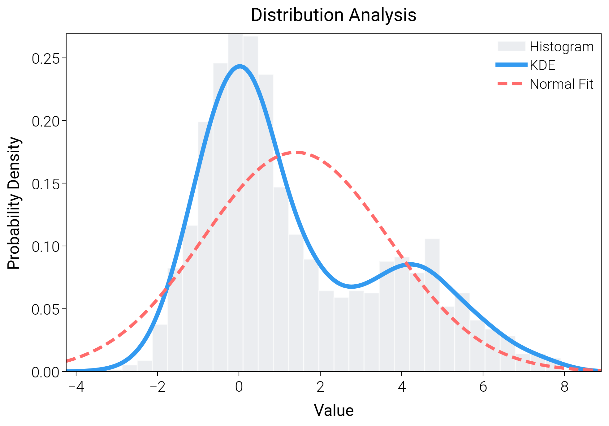
Probability Density

Plot analytic PDFs with shading and annotations so you can introduce distributions without heavy math.

import matplotlib.pyplot as plt
import numpy as np
from scipy import stats

import dartwork_mpl as dm

# Apply scientific style
dm.style.use("scientific")

# Generate synthetic data
np.random.seed(42)
data = np.concatenate(
    [np.random.normal(0, 1, 1000), np.random.normal(4, 1.5, 500)]
)

fig = plt.figure(figsize=(dm.cm2in(10), dm.cm2in(7)), dpi=300)
gs = fig.add_gridspec(1, 1, left=0.15, right=0.95, top=0.92, bottom=0.15)
ax = fig.add_subplot(gs[0, 0])

# Histogram
# Use 'density=True' to normalize
n, bins, patches = ax.hist(
    data,
    bins=30,
    density=True,
    color="oc.gray3",
    alpha=0.6,
    edgecolor="white",
    label="Histogram",
)

# Kernel Density Estimation (KDE)
kde = stats.gaussian_kde(data)
x_grid = np.linspace(data.min() - 1, data.max() + 1, 200)
ax.plot(x_grid, kde(x_grid), color="oc.blue5", lw=2, label="KDE")

# Normal Distribution Fit (for comparison)
mu, std = stats.norm.fit(data)
p = stats.norm.pdf(x_grid, mu, std)
ax.plot(x_grid, p, color="oc.red5", lw=1.5, linestyle="--", label="Normal Fit")

ax.set_xlabel("Value", fontsize=dm.fs(0))
ax.set_ylabel("Probability Density", fontsize=dm.fs(0))
ax.set_title("Distribution Analysis", fontsize=dm.fs(1))
ax.legend(fontsize=dm.fs(-1), loc="best", ncol=1)

dm.simple_layout(fig, gs=gs)
plt.show()