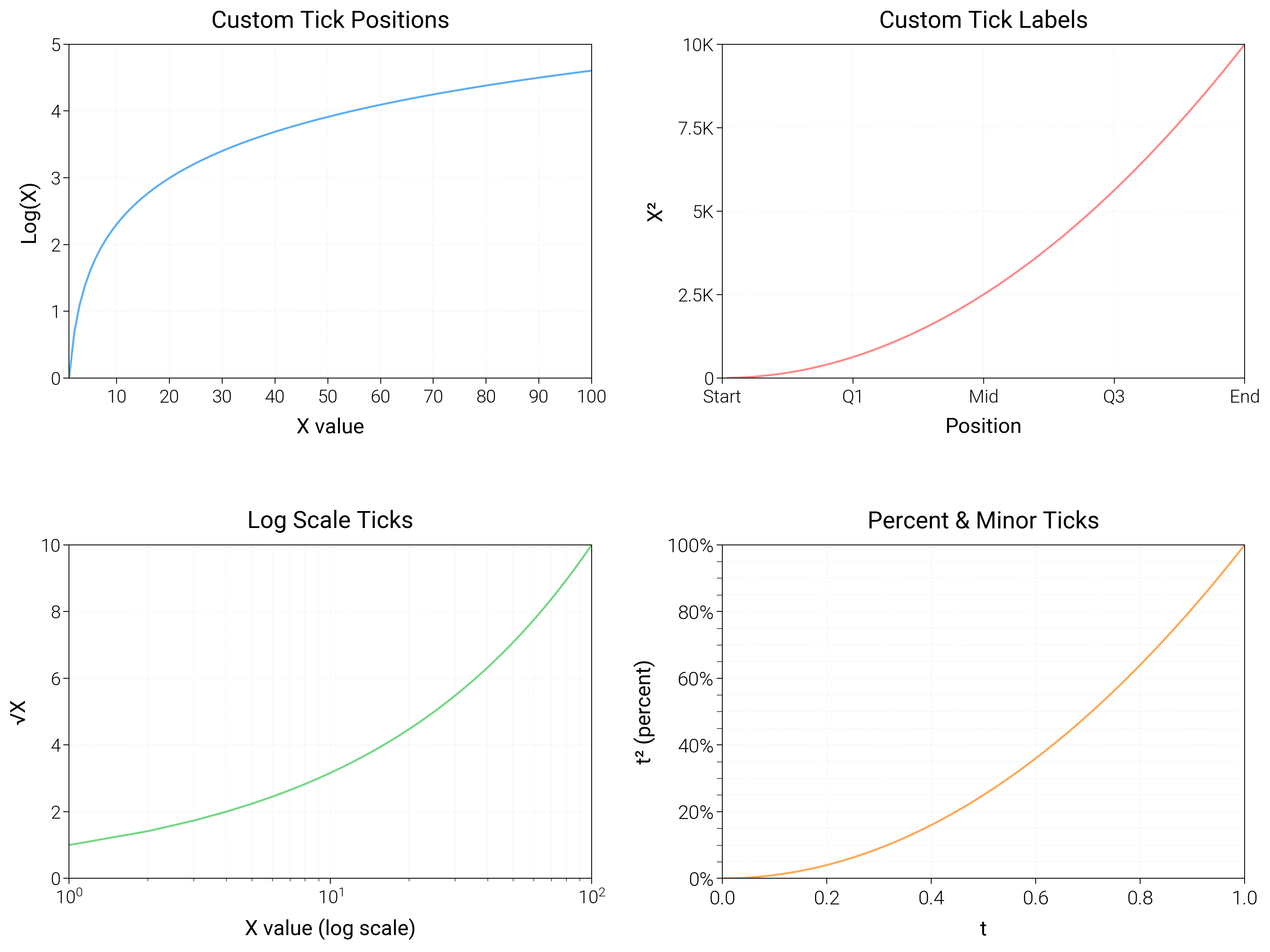
Custom Ticks

Control tick placement and formatting, from numeric to log scales, with custom formatters.

import matplotlib.pyplot as plt
import matplotlib.ticker as ticker
import numpy as np

import dartwork_mpl as dm

# Apply scientific style preset
# Default: font.size=7.5, lines.linewidth=0.5, axes.linewidth=0.3
dm.style.use("scientific")

# Generate sample data
x = np.linspace(1, 100, 100)
y1 = np.log(x)
y2 = x**2
y3 = np.sqrt(x)

# Create figure (square-ish): 16 cm wide, 12 cm tall
fig = plt.figure(figsize=(dm.cm2in(16), dm.cm2in(12)), dpi=300)

# Create GridSpec for 4 subplots (2x2)
gs = fig.add_gridspec(
    nrows=2,
    ncols=2,
    left=0.08,
    right=0.98,
    top=0.92,
    bottom=0.12,
    wspace=0.25,
    hspace=0.5,
)

# Panel A: Custom tick positions
ax1 = fig.add_subplot(gs[0, 0])
ax1.plot(x, y1, color="oc.blue5", lw=0.7, alpha=0.8)
# Explicit tick positions: [10, 20, 30, 40, 50, 60, 70, 80, 90, 100]
ax1.set_xticks([10, 20, 30, 40, 50, 60, 70, 80, 90, 100])
ax1.set_yticks([0, 1, 2, 3, 4, 5])
ax1.tick_params(axis="both", labelsize=dm.fs(-1))
ax1.set_xlabel("X value", fontsize=dm.fs(0))
ax1.set_ylabel("Log(X)", fontsize=dm.fs(0))
ax1.set_title("Custom Tick Positions", fontsize=dm.fs(1))
ax1.grid(True, linestyle="--", linewidth=0.3, alpha=0.3)

# Panel B: Custom tick labels
ax2 = fig.add_subplot(gs[0, 1])
ax2.plot(x, y2, color="oc.red5", lw=0.7, alpha=0.8)
# Explicit tick positions and custom labels
tick_positions = [0, 25, 50, 75, 100]
tick_labels = ["Start", "Q1", "Mid", "Q3", "End"]
ax2.set_xticks(tick_positions)
ax2.set_xticklabels(tick_labels, fontsize=dm.fs(-1))
ax2.set_yticks([0, 2500, 5000, 7500, 10000])
ax2.set_yticklabels(["0", "2.5K", "5K", "7.5K", "10K"], fontsize=dm.fs(-1))
ax2.set_xlabel("Position", fontsize=dm.fs(0))
ax2.set_ylabel("X²", fontsize=dm.fs(0))
ax2.set_title("Custom Tick Labels", fontsize=dm.fs(1))
ax2.grid(True, linestyle="--", linewidth=0.3, alpha=0.3)

# Panel C: Log scale ticks
ax3 = fig.add_subplot(gs[1, 0])
ax3.plot(x, y3, color="oc.green5", lw=0.7, alpha=0.8)
# Set log scale: basex=10
ax3.set_xscale("log")
# Use LogLocator for better tick spacing
ax3.xaxis.set_major_locator(ticker.LogLocator(base=10, numticks=5))
ax3.xaxis.set_minor_locator(
    ticker.LogLocator(base=10, subs=np.arange(2, 10), numticks=10)
)
# Format log scale labels
ax3.xaxis.set_major_formatter(ticker.LogFormatterSciNotation())
ax3.set_yticks([0, 2, 4, 6, 8, 10])
ax3.tick_params(axis="both", labelsize=dm.fs(-1))
ax3.set_xlabel("X value (log scale)", fontsize=dm.fs(0))
ax3.set_ylabel("√X", fontsize=dm.fs(0))
ax3.set_title("Log Scale Ticks", fontsize=dm.fs(1))
ax3.grid(True, linestyle="--", linewidth=0.3, alpha=0.3, which="both")

# Panel D: Secondary ticks and percent formatter
ax4 = fig.add_subplot(gs[1, 1])
t = np.linspace(0, 1, 100)
ax4.plot(t, t**2, color="oc.orange5", lw=0.7, alpha=0.8)
ax4.yaxis.set_major_formatter(ticker.PercentFormatter(1.0, decimals=0))
ax4.yaxis.set_minor_locator(ticker.MultipleLocator(0.05))
ax4.tick_params(axis="y", which="minor", length=2)
ax4.set_xlabel("t", fontsize=dm.fs(0))
ax4.set_ylabel("t² (percent)", fontsize=dm.fs(0))
ax4.set_title("Percent & Minor Ticks", fontsize=dm.fs(1))
ax4.grid(True, linestyle="--", linewidth=0.3, alpha=0.3, which="both")

# Optimize layout
dm.simple_layout(fig, gs=gs)

# Show plot
plt.show()