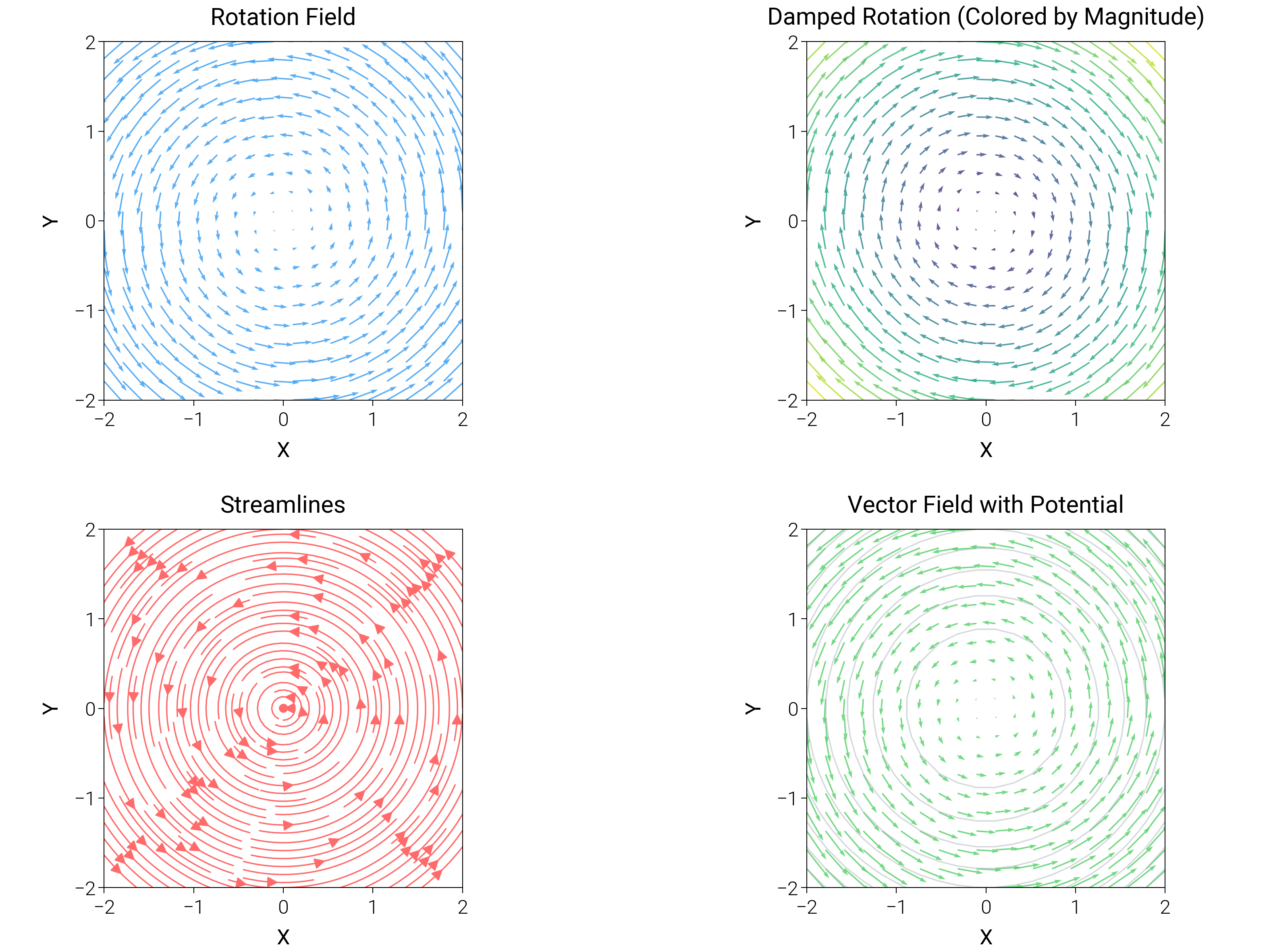
Advanced Vector Fields

Blend streamlines, contour backgrounds, and reference arrows to explain complex vector fields.

import matplotlib.pyplot as plt
import numpy as np

import dartwork_mpl as dm

# Apply scientific style preset
dm.style.use("scientific")

# Create meshgrid
x = np.linspace(-2, 2, 20)
y = np.linspace(-2, 2, 20)
X, Y = np.meshgrid(x, y)

# Define different vector fields
U1 = -Y
V1 = X
U2 = Y
V2 = -X - 0.1 * Y
U3 = np.sin(X) * np.cos(Y)
V3 = -np.cos(X) * np.sin(Y)

# Create figure
fig = plt.figure(figsize=(dm.cm2in(16), dm.cm2in(12)), dpi=300)

# Create GridSpec for 2x2 subplots
gs = fig.add_gridspec(
    nrows=2,
    ncols=2,
    left=0.07,
    right=0.95,
    top=0.95,
    bottom=0.08,
    wspace=0.24,
    hspace=0.36,
)

# Panel A: Basic quiver plot
ax1 = fig.add_subplot(gs[0, 0])
ax1.quiver(X, Y, U1, V1, alpha=0.8, width=0.004, scale=25, color="oc.blue5")
ax1.set_xlabel("X", fontsize=dm.fs(0))
ax1.set_ylabel("Y", fontsize=dm.fs(0))
ax1.set_title("Rotation Field", fontsize=dm.fs(1))
ax1.set_aspect("equal")
ax1.set_xticks([-2, -1, 0, 1, 2])
ax1.set_yticks([-2, -1, 0, 1, 2])

# Panel B: Colored by magnitude
ax2 = fig.add_subplot(gs[0, 1])
magnitude = np.sqrt(U2**2 + V2**2)
ax2.quiver(
    X, Y, U2, V2, magnitude, alpha=0.8, width=0.004, scale=25, cmap="viridis"
)
ax2.set_xlabel("X", fontsize=dm.fs(0))
ax2.set_ylabel("Y", fontsize=dm.fs(0))
ax2.set_title("Damped Rotation (Colored by Magnitude)", fontsize=dm.fs(1))
ax2.set_aspect("equal")
ax2.set_xticks([-2, -1, 0, 1, 2])
ax2.set_yticks([-2, -1, 0, 1, 2])

# Panel C: Streamplot
ax3 = fig.add_subplot(gs[1, 0])
x_fine = np.linspace(-2, 2, 100)
y_fine = np.linspace(-2, 2, 100)
X_fine, Y_fine = np.meshgrid(x_fine, y_fine)
U_fine = -Y_fine
V_fine = X_fine
strm = ax3.streamplot(
    X_fine,
    Y_fine,
    U_fine,
    V_fine,
    color="oc.red5",
    linewidth=0.5,
    density=1.5,
    arrowsize=0.8,
)
ax3.set_xlabel("X", fontsize=dm.fs(0))
ax3.set_ylabel("Y", fontsize=dm.fs(0))
ax3.set_title("Streamlines", fontsize=dm.fs(1))
ax3.set_aspect("equal")
ax3.set_xticks([-2, -1, 0, 1, 2])
ax3.set_yticks([-2, -1, 0, 1, 2])

# Panel D: Vector field with contour
ax4 = fig.add_subplot(gs[1, 1])
# Potential function
potential = 0.5 * (X**2 + Y**2)
contour = ax4.contour(
    X, Y, potential, levels=10, colors="oc.gray5", linewidths=0.5, alpha=0.5
)
ax4.quiver(X, Y, U1, V1, alpha=0.8, width=0.004, scale=25, color="oc.green5")
ax4.set_xlabel("X", fontsize=dm.fs(0))
ax4.set_ylabel("Y", fontsize=dm.fs(0))
ax4.set_title("Vector Field with Potential", fontsize=dm.fs(1))
ax4.set_aspect("equal")
ax4.set_xticks([-2, -1, 0, 1, 2])
ax4.set_yticks([-2, -1, 0, 1, 2])

# Optimize layout
dm.simple_layout(fig, gs=gs)

# Save and show plot
plt.show()