Dynamic Particle Systems

Create mesmerizing particle system visualizations with motion trails, gravitational effects, and beautiful color gradients using dartwork-mpl.

import matplotlib.patheffects as path_effects
import matplotlib.pyplot as plt
import numpy as np
from matplotlib.colors import LinearSegmentedColormap
from matplotlib.patches import Circle

import dartwork_mpl as dm

np.random.seed(42)

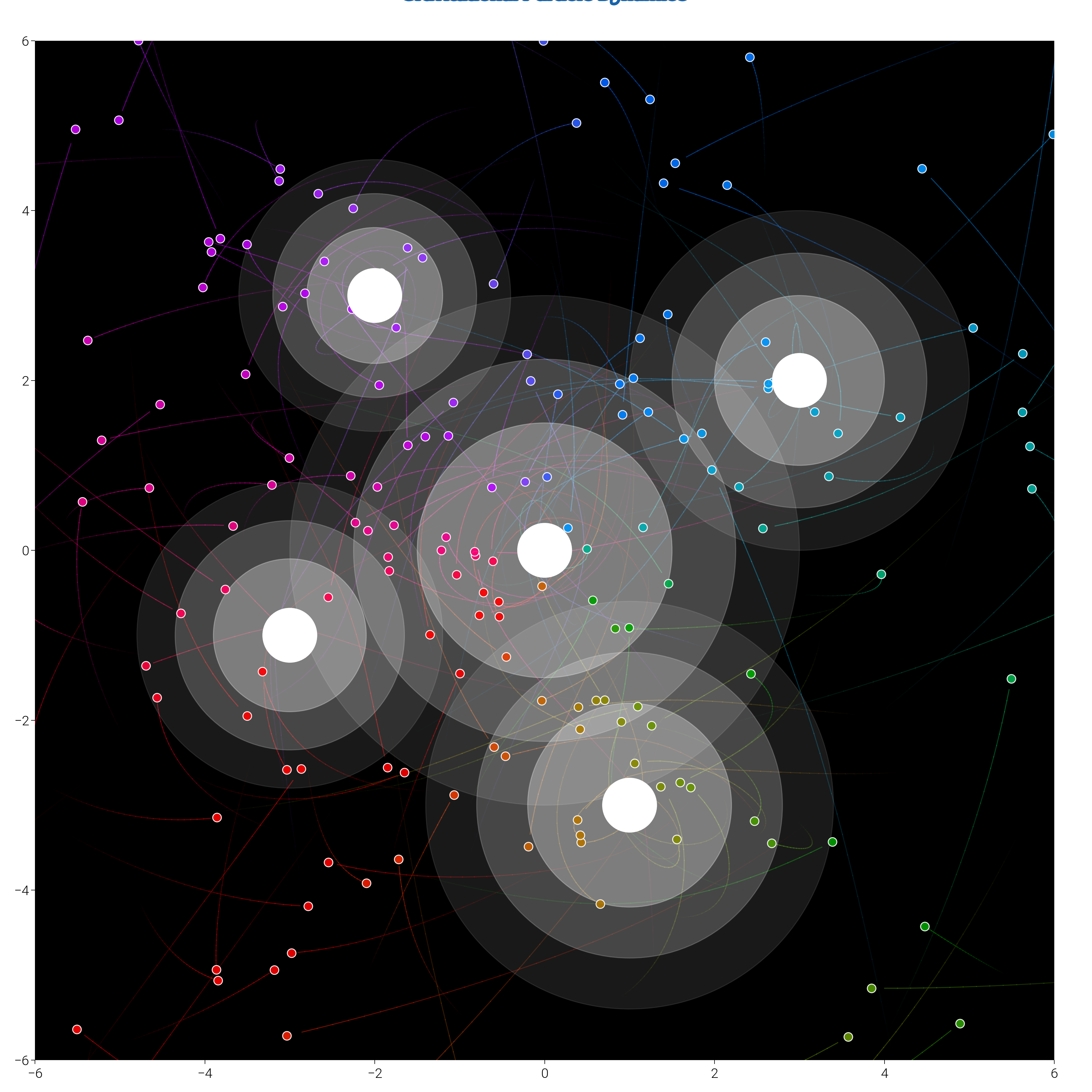
Gravitational Particle Swarm

Simulate particles attracted to multiple gravity wells with colorful trails.

dm.style.use("scientific")

fig, ax = plt.subplots(figsize=(dm.cm2in(20), dm.cm2in(20)))

# Define gravity wells
wells = [
    (0, 0, 1.5),  # (x, y, strength)
    (3, 2, 1.0),
    (-2, 3, 0.8),
    (1, -3, 1.2),
    (-3, -1, 0.9),
]

# Initialize particles
n_particles = 200
particles_x = np.random.randn(n_particles) * 4
particles_y = np.random.randn(n_particles) * 4
particles_vx = np.random.randn(n_particles) * 0.1
particles_vy = np.random.randn(n_particles) * 0.1

# Store trails
trail_length = 30
trails_x = np.zeros((n_particles, trail_length))
trails_y = np.zeros((n_particles, trail_length))

# Simulate motion
for step in range(trail_length):
    # Update trails
    trails_x[:, step] = particles_x
    trails_y[:, step] = particles_y

    # Calculate forces from gravity wells
    fx = np.zeros(n_particles)
    fy = np.zeros(n_particles)

    for wx, wy, strength in wells:
        dx = wx - particles_x
        dy = wy - particles_y
        r = np.sqrt(dx**2 + dy**2) + 0.1  # Avoid division by zero
        force = strength / r**2
        fx += force * dx / r
        fy += force * dy / r

    # Update velocities and positions
    particles_vx += fx * 0.01
    particles_vy += fy * 0.01
    particles_vx *= 0.99  # Damping
    particles_vy *= 0.99
    particles_x += particles_vx
    particles_y += particles_vy

# Draw trails with gradient
for i in range(n_particles):
    # Color based on particle position
    angle = np.arctan2(particles_y[i], particles_x[i])
    hue = (angle + np.pi) / (2 * np.pi) * 360
    color = dm.oklch(0.6, 0.3, hue)

    # Draw trail with fading effect
    for j in range(trail_length - 1):
        alpha = j / trail_length * 0.5
        ax.plot(
            [trails_x[i, j], trails_x[i, j + 1]],
            [trails_y[i, j], trails_y[i, j + 1]],
            color=color.to_hex(),
            alpha=alpha,
            lw=0.5,
        )

    # Draw particle
    ax.scatter(
        particles_x[i],
        particles_y[i],
        s=20,
        c=[color.to_hex()],
        edgecolors="white",
        linewidths=0.5,
        alpha=0.9,
        zorder=10,
    )

# Draw gravity wells
for wx, wy, strength in wells:
    # Outer glow
    for r, alpha in [(2, 0.1), (1.5, 0.2), (1, 0.3)]:
        circle = Circle(
            (wx, wy), r * strength, color="white", alpha=alpha, zorder=5
        )
        ax.add_patch(circle)
    # Core
    circle = Circle(
        (wx, wy),
        0.3,
        color="white",
        edgecolor="oc.blue5",
        linewidth=2,
        zorder=15,
    )
    ax.add_patch(circle)

# Styling
ax.set_xlim(-6, 6)
ax.set_ylim(-6, 6)
ax.set_aspect("equal")
dm.hide_all_spines(ax)
ax.set_facecolor("black")

# Title
title = ax.text(
    0,
    6.5,
    "Gravitational Particle Dynamics",
    ha="center",
    fontsize=dm.fs(3),
    color="white",
    weight="bold",
)
title.set_path_effects(
    [path_effects.withStroke(linewidth=3, foreground="oc.blue9")]
)

dm.simple_layout(fig)

/home/runner/work/dartwork-mpl/dartwork-mpl/docs/examples_source/06_creative_visualizations/plot_particle_systems.py:115: UserWarning: Setting the 'color' property will override the edgecolor or facecolor properties.
  circle = Circle(

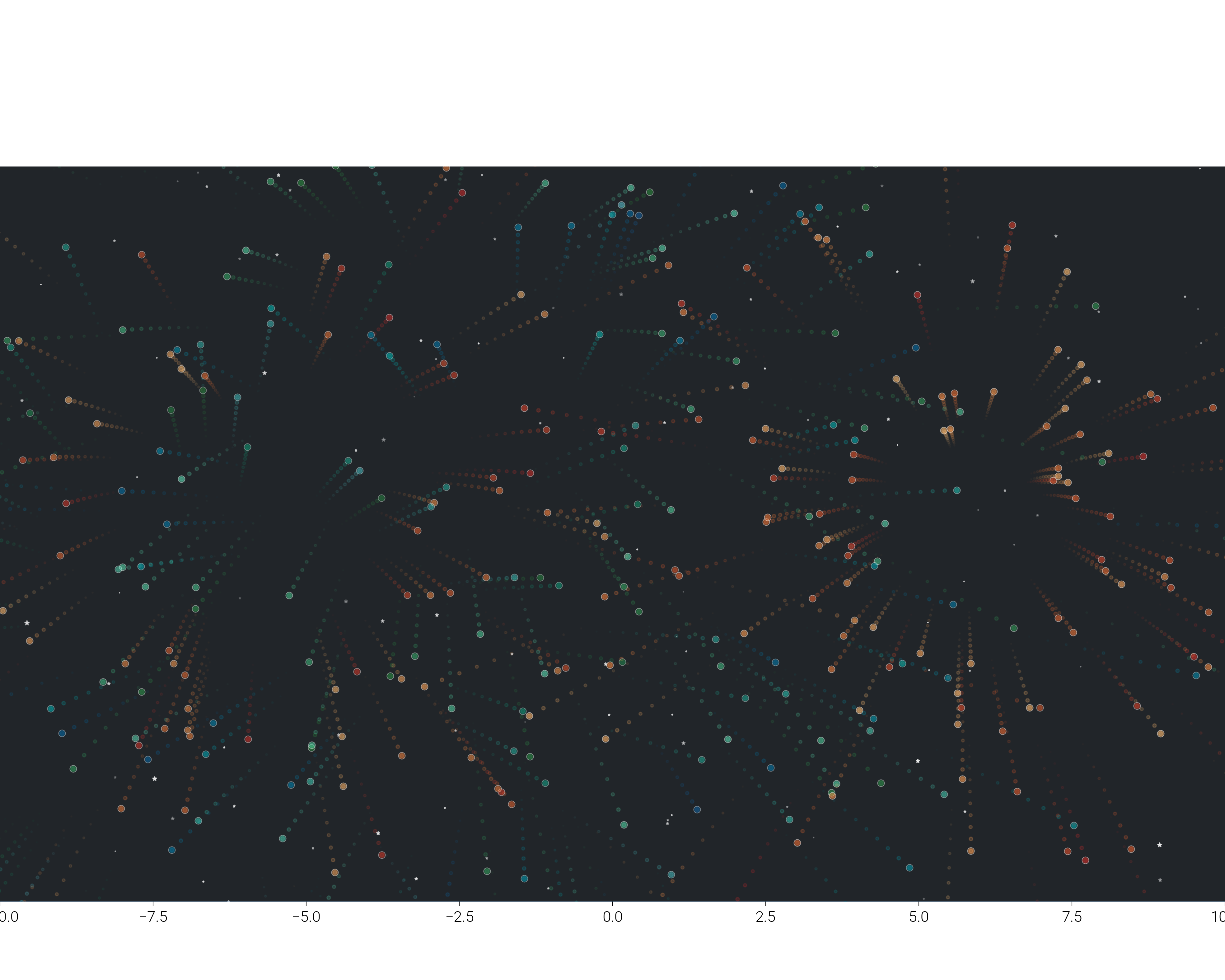
Fireworks Explosion Simulation

Create a spectacular fireworks display with realistic particle physics.

fig, ax = plt.subplots(figsize=(dm.cm2in(20), dm.cm2in(16)))

# Create multiple firework explosions
n_fireworks = 5
explosion_data = []

for _fw in range(n_fireworks):
    # Random explosion parameters
    center_x = np.random.uniform(-8, 8)
    center_y = np.random.uniform(2, 8)
    n_particles_fw = np.random.randint(80, 150)
    explosion_time = np.random.uniform(0, 0.5)

    # Color scheme for this firework
    color_start = (
        f"oc.{np.random.choice(['red', 'blue', 'green', 'yellow', 'purple'])}9"
    )
    color_end = (
        f"oc.{np.random.choice(['orange', 'cyan', 'pink', 'teal', 'violet'])}3"
    )
    colors = dm.cspace(color_start, color_end, n=n_particles_fw)

    # Generate explosion particles
    angles = np.random.uniform(0, 2 * np.pi, n_particles_fw)
    speeds = np.random.exponential(2, n_particles_fw) + np.random.uniform(1, 3)

    explosion_data.append(
        {
            "center": (center_x, center_y),
            "particles": n_particles_fw,
            "angles": angles,
            "speeds": speeds,
            "colors": colors,
            "time": explosion_time,
        }
    )

# Draw fireworks at different stages
for fw_data in explosion_data:
    center_x, center_y = fw_data["center"]

    # Calculate particle positions (with gravity)
    t = 2 - fw_data["time"]  # Time since explosion
    gravity = 0.5

    for i in range(fw_data["particles"]):
        angle = fw_data["angles"][i]
        speed = fw_data["speeds"][i]

        # Physics calculation
        x = center_x + speed * np.cos(angle) * t
        y = center_y + speed * np.sin(angle) * t - 0.5 * gravity * t**2

        # Particle trail
        trail_steps = 10
        for j in range(trail_steps):
            t_trail = t - j * 0.05
            if t_trail > 0:
                x_trail = center_x + speed * np.cos(angle) * t_trail
                y_trail = (
                    center_y
                    + speed * np.sin(angle) * t_trail
                    - 0.5 * gravity * t_trail**2
                )

                alpha = (1 - j / trail_steps) * (1 - t / 3) * 0.5
                size = 3 * (1 - j / trail_steps)

                ax.scatter(
                    x_trail,
                    y_trail,
                    s=size,
                    c=[fw_data["colors"][i].to_hex()],
                    alpha=alpha,
                )

        # Main particle
        if y > -2:  # Don't show if fallen too far
            alpha = max(0, 1 - t / 3)
            ax.scatter(
                x,
                y,
                s=10,
                c=[fw_data["colors"][i].to_hex()],
                edgecolors="white",
                linewidths=0.3,
                alpha=alpha,
                zorder=10,
            )

    # Explosion flash
    if fw_data["time"] < 0.1:
        flash = Circle(
            (center_x, center_y),
            1,
            color="white",
            alpha=0.5 - fw_data["time"] * 5,
        )
        ax.add_patch(flash)

# Add sparkling stars
n_stars = 100
stars_x = np.random.uniform(-10, 10, n_stars)
stars_y = np.random.uniform(-2, 10, n_stars)
star_sizes = np.random.exponential(1, n_stars)
star_alphas = np.random.uniform(0.2, 0.8, n_stars)

ax.scatter(
    stars_x, stars_y, s=star_sizes, c="white", alpha=star_alphas, marker="*"
)

# Ground reflection effect
ax.fill_between([-10, 10], -2, -2, color="oc.blue9", alpha=0.3)

# Styling
ax.set_xlim(-10, 10)
ax.set_ylim(-2, 10)
ax.set_aspect("equal")
dm.hide_all_spines(ax)
ax.set_facecolor("oc.gray9")

# Title
ax.text(
    0,
    -3,
    "Fireworks Celebration",
    ha="center",
    fontsize=dm.fs(3),
    color="white",
    weight="bold",
)

dm.simple_layout(fig)

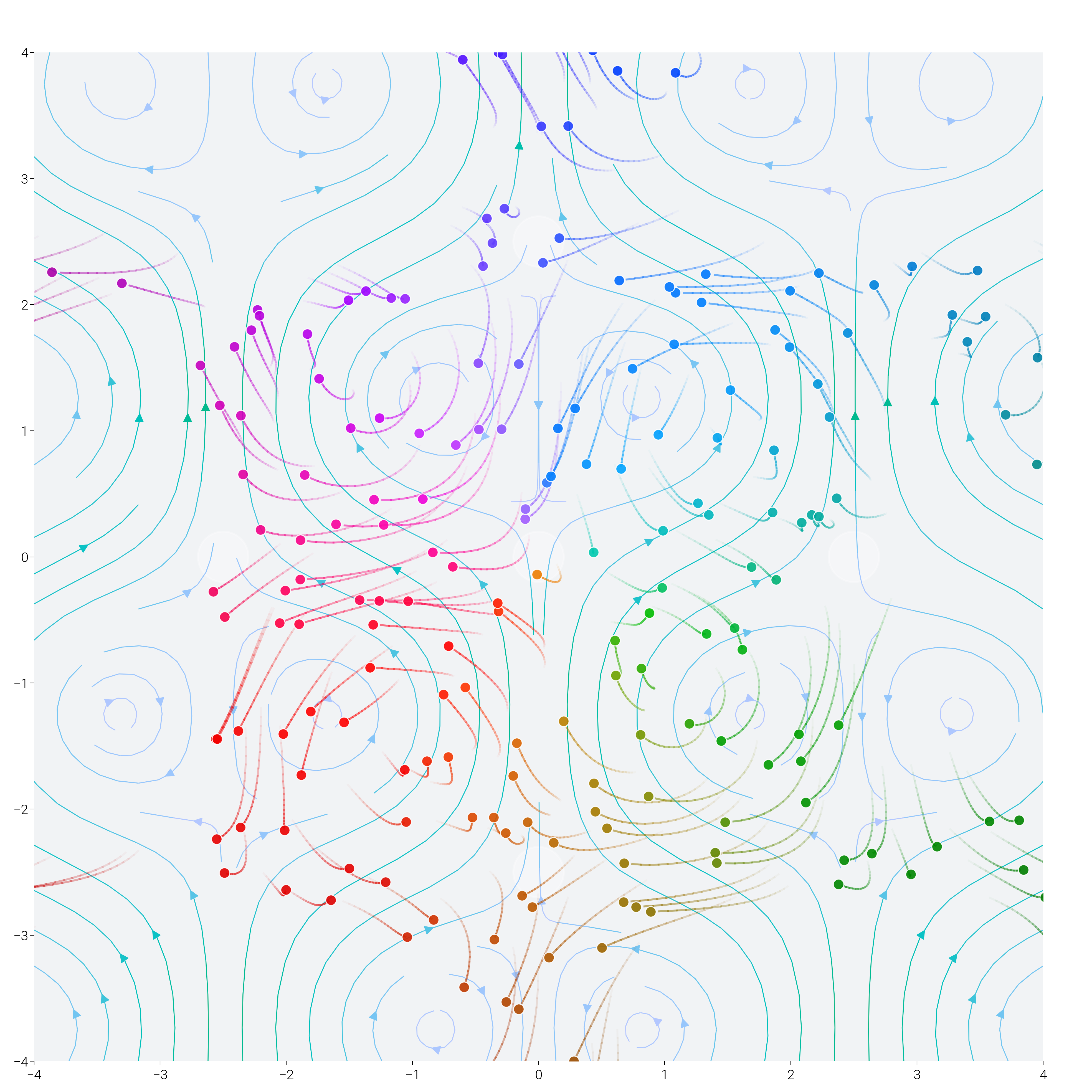
Particle Flow Field

Create an organic flow field with particles following vector forces.

fig, ax = plt.subplots(figsize=(dm.cm2in(20), dm.cm2in(20)))


# Create flow field function
def flow_field(x, y, t=0):
    """Generate flow vectors based on position"""
    u = np.sin(np.pi * x * 0.4) * np.cos(np.pi * y * 0.4) + 0.5 * np.sin(t)
    v = -np.cos(np.pi * x * 0.4) * np.sin(np.pi * y * 0.4) + 0.5 * np.cos(t)
    return u, v


# Initialize particle grid
grid_size = 15
x_grid = np.linspace(-3, 3, grid_size)
y_grid = np.linspace(-3, 3, grid_size)

# Create particles at grid intersections with some randomness
particles = []
for x in x_grid:
    for y in y_grid:
        particles.append(
            {
                "x": x + np.random.randn() * 0.1,
                "y": y + np.random.randn() * 0.1,
                "trail": [],
            }
        )

# Simulate particle movement
n_steps = 50
dt = 0.05

for step in range(n_steps):
    for particle in particles:
        # Get flow at particle position
        u, v = flow_field(particle["x"], particle["y"], step * 0.1)

        # Store current position in trail
        particle["trail"].append((particle["x"], particle["y"]))

        # Update position
        particle["x"] += u * dt
        particle["y"] += v * dt

        # Keep trail limited
        if len(particle["trail"]) > 20:
            particle["trail"].pop(0)

# Draw flow visualization
# Background flow field
x_bg = np.linspace(-4, 4, 30)
y_bg = np.linspace(-4, 4, 30)
X_bg, Y_bg = np.meshgrid(x_bg, y_bg)
U_bg, V_bg = flow_field(X_bg, Y_bg)
speed = np.sqrt(U_bg**2 + V_bg**2)

# Create custom colormap
colors_flow = dm.cspace("oc.indigo2", "oc.teal6", n=256)
flow_cmap = LinearSegmentedColormap.from_list(
    "flow", [c.to_hex() for c in colors_flow]
)

# Stream plot
strm = ax.streamplot(
    X_bg,
    Y_bg,
    U_bg,
    V_bg,
    color=speed,
    cmap=flow_cmap,
    linewidth=0.5,
    density=1,
)

# Draw particles and trails
for particle in particles:
    # Color based on position
    r = np.sqrt(particle["x"] ** 2 + particle["y"] ** 2)
    hue = (np.arctan2(particle["y"], particle["x"]) + np.pi) / (2 * np.pi) * 360
    color = dm.oklch(0.7 - r * 0.05, 0.3, hue)

    # Draw trail
    if len(particle["trail"]) > 1:
        for i in range(len(particle["trail"]) - 1):
            alpha = i / len(particle["trail"]) * 0.6
            ax.plot(
                [particle["trail"][i][0], particle["trail"][i + 1][0]],
                [particle["trail"][i][1], particle["trail"][i + 1][1]],
                color=color.to_hex(),
                alpha=alpha,
                lw=1,
            )

    # Draw particle
    ax.scatter(
        particle["x"],
        particle["y"],
        s=30,
        c=[color.to_hex()],
        edgecolors="white",
        linewidths=0.5,
        alpha=0.9,
        zorder=10,
    )

# Add vortex centers
vortices = [(0, 0), (2.5, 0), (-2.5, 0), (0, 2.5), (0, -2.5)]
for vx, vy in vortices:
    circle = Circle(
        (vx, vy),
        0.2,
        color="white",
        alpha=0.3,
        edgecolor="oc.blue5",
        linewidth=1,
    )
    ax.add_patch(circle)

# Styling
ax.set_xlim(-4, 4)
ax.set_ylim(-4, 4)
ax.set_aspect("equal")
dm.hide_all_spines(ax)
ax.set_facecolor("oc.gray1")

# Title
ax.text(
    0,
    4.5,
    "Particle Flow Dynamics",
    ha="center",
    fontsize=dm.fs(3),
    color="white",
    weight="bold",
)

dm.simple_layout(fig)

/home/runner/work/dartwork-mpl/dartwork-mpl/docs/examples_source/06_creative_visualizations/plot_particle_systems.py:402: UserWarning: Setting the 'color' property will override the edgecolor or facecolor properties.
  circle = Circle(

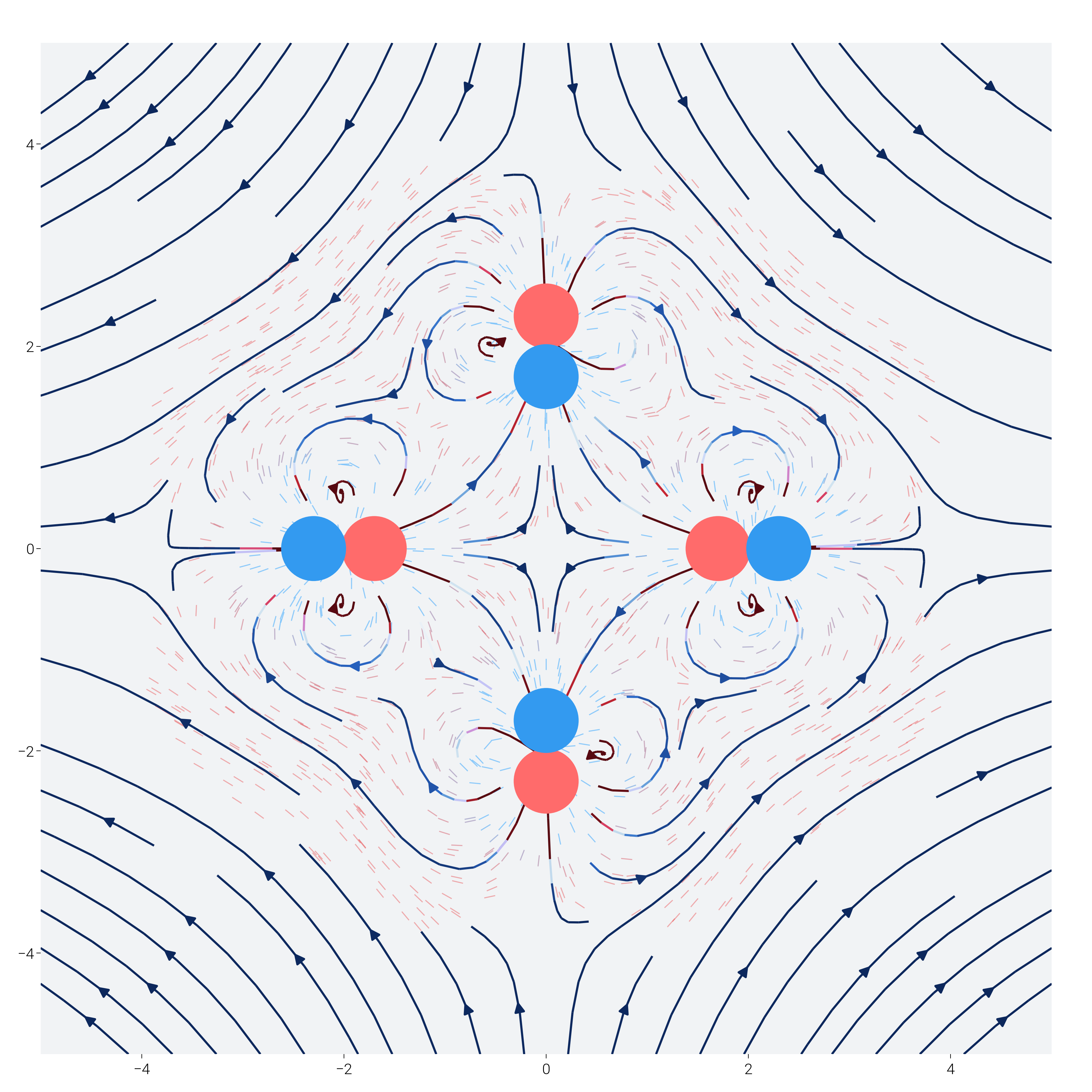
Magnetic Field Visualization

Visualize magnetic field lines with iron filing-like particles.

fig, ax = plt.subplots(figsize=(dm.cm2in(18), dm.cm2in(18)))

# Define magnetic dipoles
dipoles = [
    {"pos": (-2, 0), "moment": (1, 0), "strength": 2},
    {"pos": (2, 0), "moment": (-1, 0), "strength": 2},
    {"pos": (0, 2), "moment": (0, 1), "strength": 1.5},
    {"pos": (0, -2), "moment": (0, -1), "strength": 1.5},
]


# Calculate magnetic field
def magnetic_field(x, y, dipoles):
    Bx, By = 0, 0
    for dipole in dipoles:
        dx = x - dipole["pos"][0]
        dy = y - dipole["pos"][1]
        r = np.sqrt(dx**2 + dy**2) + 0.01

        # Dipole field calculation (simplified)
        mx, my = dipole["moment"]
        strength = dipole["strength"]

        dot = (mx * dx + my * dy) / r**2
        Bx += strength * (3 * dot * dx / r**2 - mx) / r**3
        By += strength * (3 * dot * dy / r**2 - my) / r**3

    return Bx, By


# Create grid for field lines
x = np.linspace(-5, 5, 40)
y = np.linspace(-5, 5, 40)
X, Y = np.meshgrid(x, y)

# Calculate field
Bx = np.zeros_like(X)
By = np.zeros_like(Y)
for i in range(len(x)):
    for j in range(len(y)):
        Bx[j, i], By[j, i] = magnetic_field(X[j, i], Y[j, i], dipoles)

# Field magnitude
B_mag = np.sqrt(Bx**2 + By**2)
B_mag = np.clip(B_mag, 0, 5)

# Create iron filing particles
n_filings = 3000
filings_x = np.random.uniform(-5, 5, n_filings)
filings_y = np.random.uniform(-5, 5, n_filings)

for i in range(n_filings):
    # Get field at particle position
    bx, by = magnetic_field(filings_x[i], filings_y[i], dipoles)
    b_mag = np.sqrt(bx**2 + by**2)

    if b_mag > 0.1:  # Only show if field is strong enough
        # Normalize direction
        bx, by = bx / b_mag, by / b_mag

        # Color based on field strength
        color_intensity = min(1, b_mag / 3)
        color = dm.mix_colors("oc.blue3", "oc.red7", alpha=color_intensity)

        # Draw filing as oriented line
        length = 0.1
        ax.plot(
            [filings_x[i] - bx * length / 2, filings_x[i] + bx * length / 2],
            [filings_y[i] - by * length / 2, filings_y[i] + by * length / 2],
            color=color,
            lw=0.5,
            alpha=0.4 + 0.4 * color_intensity,
        )

# Draw field lines
colors_field = dm.cspace("oc.blue5", "oc.red5", n=10)
strm = ax.streamplot(
    X,
    Y,
    Bx,
    By,
    color=B_mag,
    cmap="dc.ice_fire",
    linewidth=1,
    density=0.8,
    arrowsize=1,
)

# Draw dipoles
for dipole in dipoles:
    # North pole (red)
    north = Circle(
        (
            dipole["pos"][0] + dipole["moment"][0] * 0.3,
            dipole["pos"][1] + dipole["moment"][1] * 0.3,
        ),
        0.3,
        color="oc.red5",
        edgecolor="white",
        linewidth=2,
        zorder=20,
    )
    ax.add_patch(north)
    ax.text(
        dipole["pos"][0] + dipole["moment"][0] * 0.3,
        dipole["pos"][1] + dipole["moment"][1] * 0.3,
        "N",
        ha="center",
        va="center",
        fontsize=dm.fs(0),
        color="white",
        weight="bold",
    )

    # South pole (blue)
    south = Circle(
        (
            dipole["pos"][0] - dipole["moment"][0] * 0.3,
            dipole["pos"][1] - dipole["moment"][1] * 0.3,
        ),
        0.3,
        color="oc.blue5",
        edgecolor="white",
        linewidth=2,
        zorder=20,
    )
    ax.add_patch(south)
    ax.text(
        dipole["pos"][0] - dipole["moment"][0] * 0.3,
        dipole["pos"][1] - dipole["moment"][1] * 0.3,
        "S",
        ha="center",
        va="center",
        fontsize=dm.fs(0),
        color="white",
        weight="bold",
    )

# Styling
ax.set_xlim(-5, 5)
ax.set_ylim(-5, 5)
ax.set_aspect("equal")
dm.hide_all_spines(ax)
ax.set_facecolor("oc.gray1")

# Title
ax.text(
    0,
    5.5,
    "Magnetic Field Visualization",
    ha="center",
    fontsize=dm.fs(3),
    color="white",
    weight="bold",
)

dm.simple_layout(fig)

plt.show()

/home/runner/work/dartwork-mpl/dartwork-mpl/docs/examples_source/06_creative_visualizations/plot_particle_systems.py:529: UserWarning: Setting the 'color' property will override the edgecolor or facecolor properties.
  north = Circle(
/home/runner/work/dartwork-mpl/dartwork-mpl/docs/examples_source/06_creative_visualizations/plot_particle_systems.py:553: UserWarning: Setting the 'color' property will override the edgecolor or facecolor properties.
  south = Circle(