Musical Waveform Art

Transform audio-inspired waveforms into stunning visual art using dartwork-mpl’s color gradients and styling capabilities.

import matplotlib.pyplot as plt
import numpy as np
from matplotlib.colors import LinearSegmentedColormap
from matplotlib.patches import Rectangle

import dartwork_mpl as dm

np.random.seed(42)

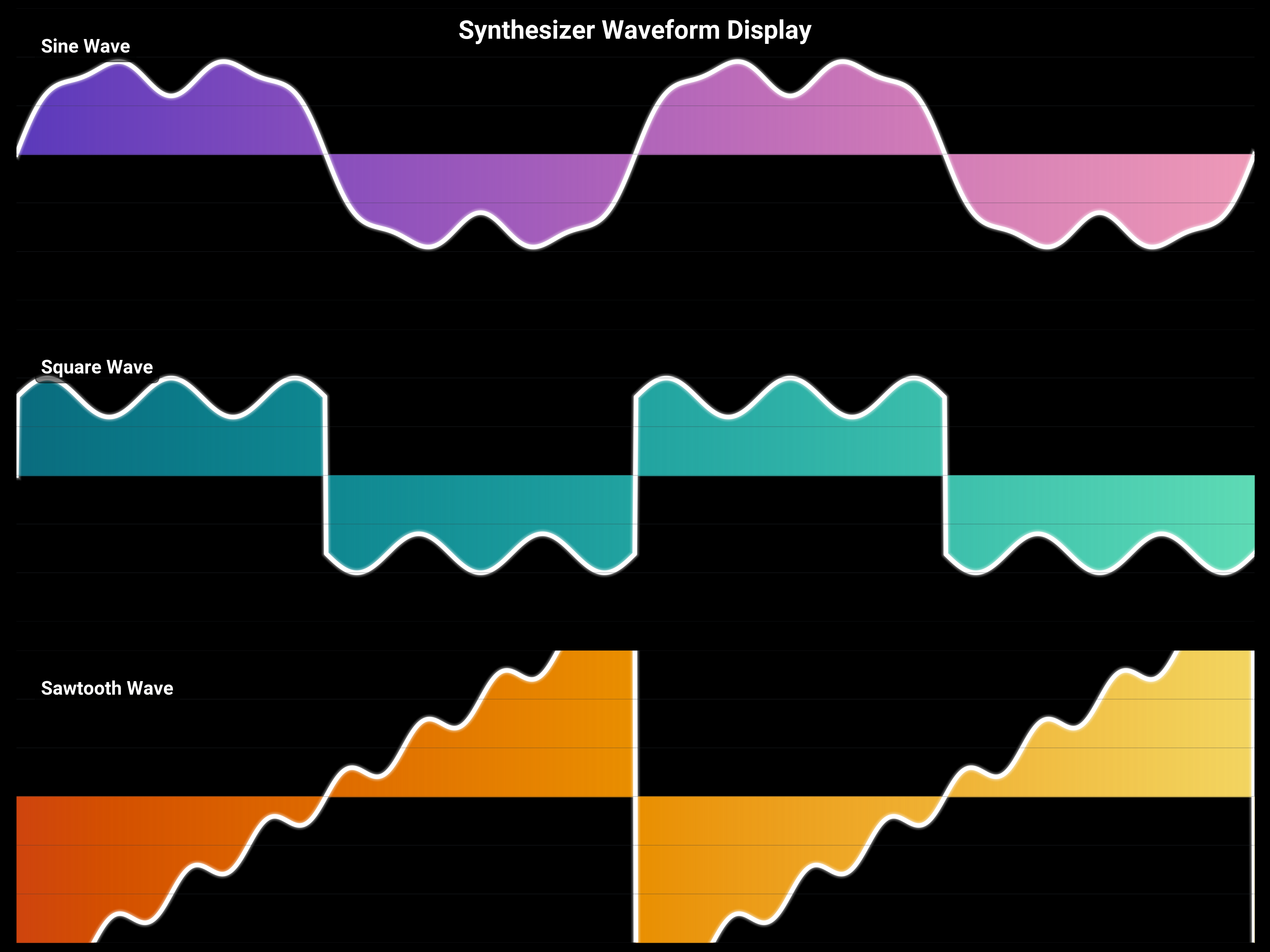
Synth Wave Visualization

Create a retro-futuristic synthesizer waveform display.

dm.style.use("scientific")

fig, axes = plt.subplots(
    3, 1, figsize=(dm.cm2in(20), dm.cm2in(15)), gridspec_kw={"hspace": 0.1}
)

# Generate waveforms
t = np.linspace(0, 4 * np.pi, 1000)

# Different wave types
waves = [
    ("Sine Wave", np.sin(t) + 0.3 * np.sin(3 * t) + 0.1 * np.sin(7 * t)),
    ("Square Wave", np.sign(np.sin(t)) * 0.8 + 0.2 * np.sin(5 * t)),
    ("Sawtooth Wave", 2 * (t / np.pi % 2 - 1) + 0.15 * np.sin(8 * t)),
]

# Color schemes for each wave
color_schemes = [
    dm.cspace("oc.violet9", "oc.pink3", n=len(t)),
    dm.cspace("oc.cyan9", "oc.teal3", n=len(t)),
    dm.cspace("oc.orange9", "oc.yellow3", n=len(t)),
]

for ax, (name, wave), colors in zip(axes, waves, color_schemes, strict=False):
    # Create gradient fill under wave
    for i in range(len(t) - 1):
        ax.fill_between(
            [t[i], t[i + 1]],
            0,
            [wave[i], wave[i + 1]],
            color=colors[i].to_hex(),
            alpha=0.7,
        )

    # Draw the wave line with glow effect
    for offset, alpha in [(3, 0.1), (2, 0.2), (1, 0.3)]:
        ax.plot(t, wave, color="white", lw=dm.lw(0.5) + offset, alpha=alpha)
    ax.plot(t, wave, color="white", lw=dm.lw(1))

    # Add wave type label
    ax.text(
        0.02,
        0.85,
        name,
        transform=ax.transAxes,
        fontsize=dm.fs(1),
        color="white",
        weight="bold",
        bbox={"boxstyle": "round,pad=0.3", "facecolor": "black", "alpha": 0.5},
    )

    # Styling
    ax.set_xlim(0, 4 * np.pi)
    ax.set_ylim(-1.5, 1.5)
    dm.hide_all_spines(ax)
    ax.set_facecolor("black")
    ax.set_xticks([])
    ax.set_yticks([])

    # Add grid lines for visual effect
    for y in np.linspace(-1.5, 1.5, 7):
        ax.axhline(y, color="oc.gray8", lw=0.3, alpha=0.3)

# Overall title
fig.suptitle(
    "Synthesizer Waveform Display",
    fontsize=dm.fs(4),
    color="white",
    weight="bold",
    y=0.98,
)
fig.patch.set_facecolor("black")

dm.simple_layout(fig)

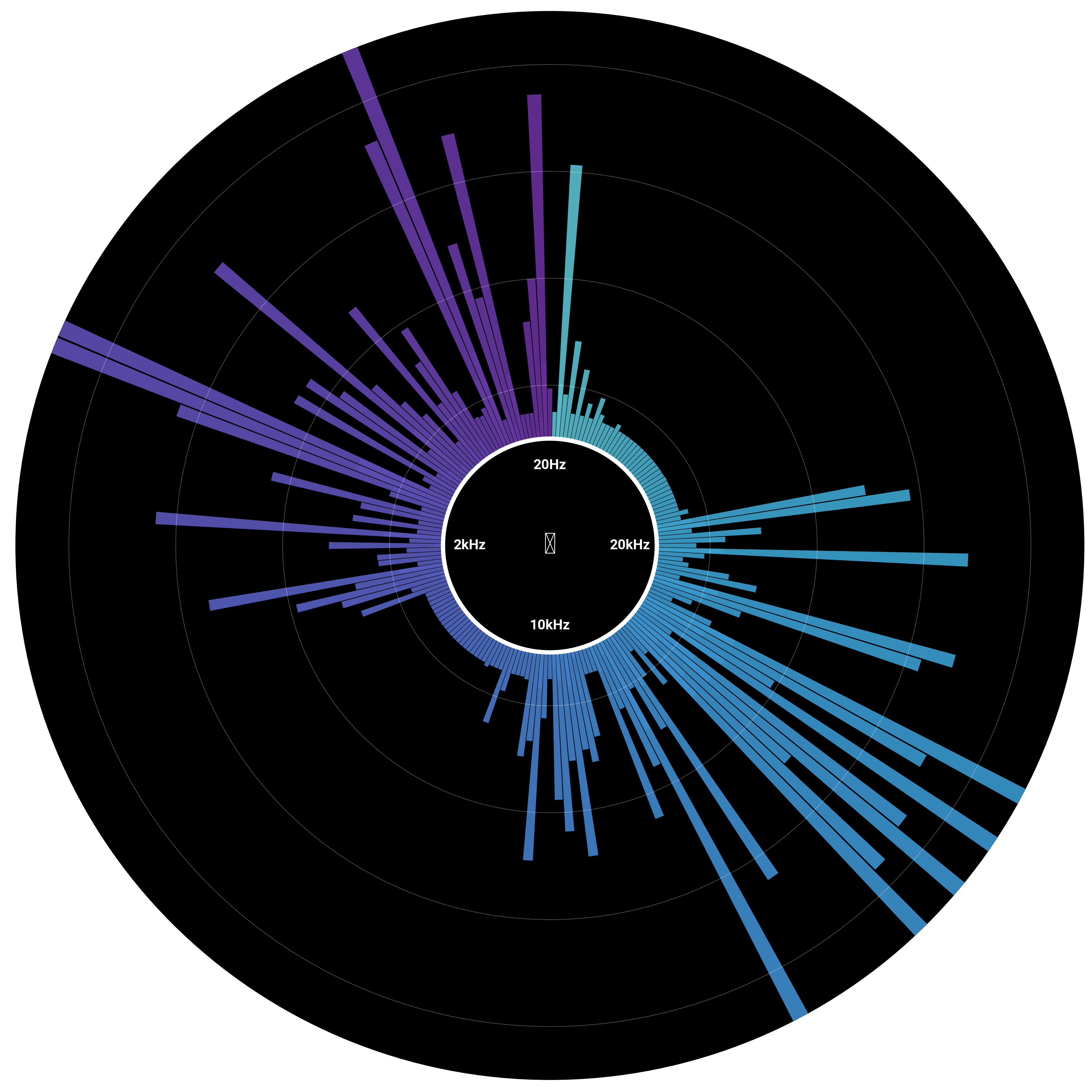
Circular Audio Spectrum Visualizer

Create a circular spectrum analyzer with radial frequency bars.

fig, ax = plt.subplots(
    figsize=(dm.cm2in(18), dm.cm2in(18)), subplot_kw={"projection": "polar"}
)

# Generate frequency data
n_frequencies = 180
frequencies = np.random.exponential(2, n_frequencies) * (
    1 + np.sin(np.linspace(0, 4 * np.pi, n_frequencies))
)
frequencies = np.clip(frequencies, 0.5, 8)

# Angular positions
theta = np.linspace(0, 2 * np.pi, n_frequencies, endpoint=False)

# Create color gradient based on frequency magnitude
colors = dm.cspace("oc.purple9", "oc.cyan3", n=n_frequencies, space="oklch")

# Draw frequency bars
bar_width = 2 * np.pi / n_frequencies * 0.9
for _i, (angle, freq, color) in enumerate(zip(theta, frequencies, colors, strict=False)):
    # Main bar
    ax.bar(
        angle,
        freq,
        width=bar_width,
        bottom=2,
        color=color.to_hex(),
        alpha=0.8,
        edgecolor="none",
    )

    # Reflection effect
    ax.bar(
        angle,
        freq * 0.3,
        width=bar_width,
        bottom=1.5,
        color=color.to_hex(),
        alpha=0.3,
        edgecolor="none",
    )

# Add center circle
circle = plt.Circle(
    (0, 0),
    2,
    transform=ax.transData._b,
    facecolor="black",
    edgecolor="white",
    linewidth=2,
)
ax.add_patch(circle)

# Add frequency labels
for angle, label in [
    (0, "20Hz"),
    (np.pi / 2, "2kHz"),
    (np.pi, "10kHz"),
    (3 * np.pi / 2, "20kHz"),
]:
    ax.text(
        angle,
        1.5,
        label,
        ha="center",
        va="center",
        fontsize=dm.fs(-1),
        color="white",
        weight="bold",
    )

# Add audio level rings
for r in [3, 5, 7, 9]:
    circle = plt.Circle(
        (0, 0),
        r,
        transform=ax.transData._b,
        fill=False,
        edgecolor="white",
        linewidth=0.3,
        alpha=0.3,
    )
    ax.add_patch(circle)

# Styling
ax.set_ylim(0, 10)
ax.set_theta_zero_location("N")
ax.set_theta_direction(1)
dm.hide_all_spines(ax)
ax.set_xticks([])
ax.set_yticks([])
ax.set_facecolor("black")

# Add central icon
ax.text(
    0,
    0,
    "♪",
    fontsize=dm.fs(6),
    ha="center",
    va="center",
    color="white",
    weight="bold",
)

dm.simple_layout(fig)

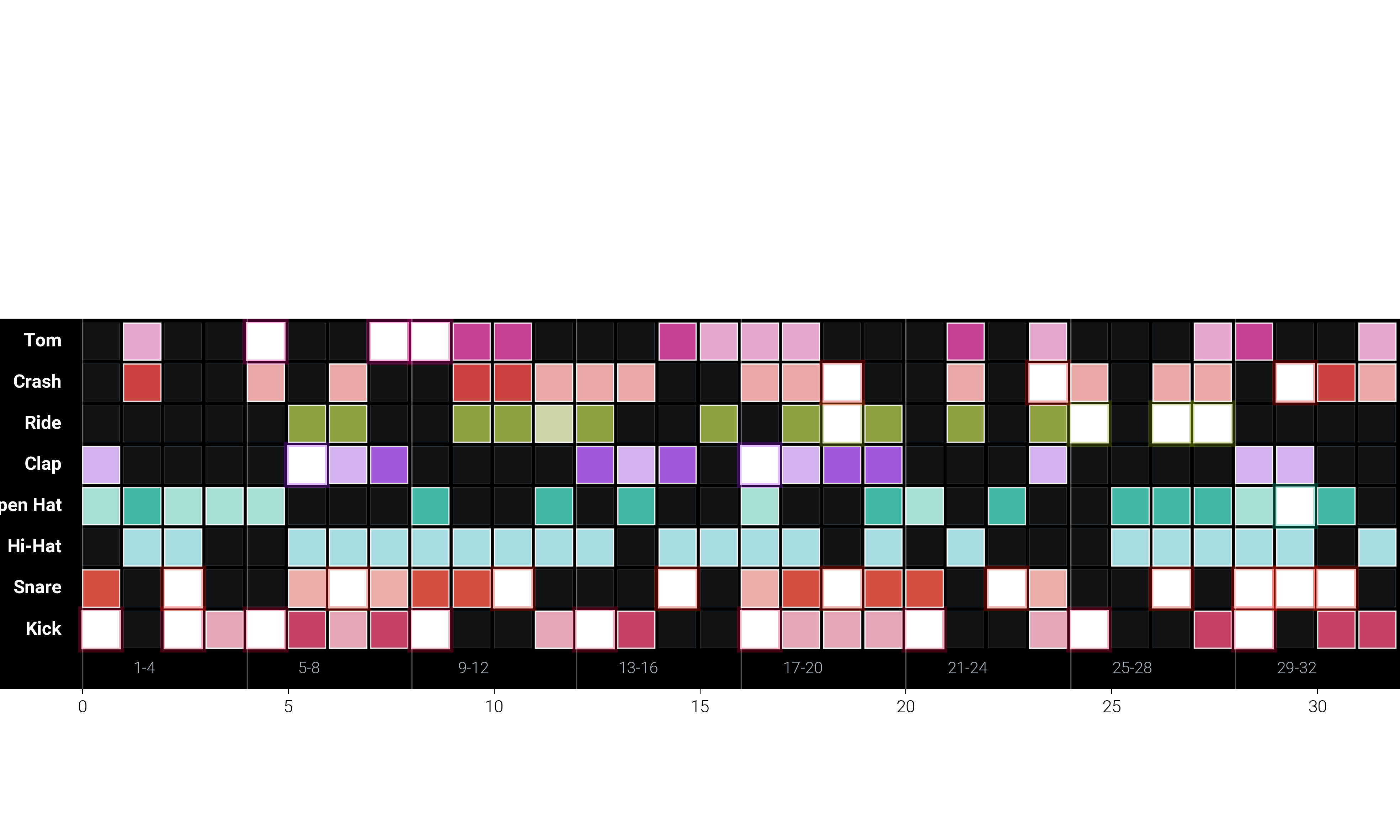
Beat Pattern Matrix

Create a drum machine-inspired beat pattern visualization.

fig, ax = plt.subplots(figsize=(dm.cm2in(20), dm.cm2in(12)))

# Define instruments and pattern
instruments = [
    "Kick",
    "Snare",
    "Hi-Hat",
    "Open Hat",
    "Clap",
    "Ride",
    "Crash",
    "Tom",
]
n_beats = 32
pattern = np.random.choice(
    [0, 0.3, 0.7, 1], size=(len(instruments), n_beats), p=[0.5, 0.2, 0.2, 0.1]
)

# Ensure some structure in the pattern
pattern[0, ::4] = 1  # Kick on downbeats
pattern[1, 2::4] = 1  # Snare on 2 and 4
pattern[2, :] = np.where(
    np.random.rand(n_beats) > 0.3, 0.7, 0
)  # Hi-hat pattern

# Create color gradients for each instrument
instrument_colors = [
    dm.oklch(0.5, 0.3, 10),  # Red for kick
    dm.oklch(0.6, 0.3, 60),  # Yellow for snare
    dm.oklch(0.7, 0.2, 200),  # Blue for hi-hat
    dm.oklch(0.7, 0.2, 180),  # Cyan for open hat
    dm.oklch(0.6, 0.3, 300),  # Purple for clap
    dm.oklch(0.65, 0.25, 120),  # Green for ride
    dm.oklch(0.5, 0.35, 40),  # Orange for crash
    dm.oklch(0.55, 0.3, 350),  # Pink for tom
]

# Draw beat grid
for i, (_instrument, color) in enumerate(zip(instruments, instrument_colors, strict=False)):
    for j in range(n_beats):
        intensity = pattern[i, j]

        if intensity > 0:
            # Create gradient effect
            rect_color = dm.mix_colors(
                color.to_hex(), "white", alpha=1 - intensity
            )

            # Main beat square
            rect = Rectangle(
                (j, i),
                0.9,
                0.9,
                facecolor=rect_color,
                edgecolor="white",
                linewidth=1 if intensity == 1 else 0.5,
                alpha=0.8 + 0.2 * intensity,
            )
            ax.add_patch(rect)

            # Add glow for strong beats
            if intensity == 1:
                glow = Rectangle(
                    (j - 0.05, i - 0.05),
                    1,
                    1,
                    facecolor="none",
                    edgecolor=color.to_hex(),
                    linewidth=2,
                    alpha=0.3,
                )
                ax.add_patch(glow)
        else:
            # Empty beat
            rect = Rectangle(
                (j, i),
                0.9,
                0.9,
                facecolor="oc.gray9",
                edgecolor="oc.gray7",
                linewidth=0.3,
                alpha=0.5,
            )
            ax.add_patch(rect)

# Add instrument labels
for i, instrument in enumerate(instruments):
    ax.text(
        -0.5,
        i + 0.45,
        instrument,
        ha="right",
        va="center",
        fontsize=dm.fs(0),
        color="white",
        weight="bold",
    )

# Add beat numbers
for j in range(0, n_beats, 4):
    ax.text(
        j + 1.5,
        -0.5,
        f"{j + 1}-{j + 4}",
        ha="center",
        va="center",
        fontsize=dm.fs(-1),
        color="oc.gray5",
    )

# Add measure indicators
for j in range(0, n_beats, 4):
    ax.axvline(j, color="white", lw=0.5, alpha=0.3)

# Styling
ax.set_xlim(-2, n_beats)
ax.set_ylim(-1, len(instruments))
ax.set_aspect("equal")
dm.hide_all_spines(ax)
ax.set_facecolor("black")

# Title
ax.text(
    n_beats / 2,
    len(instruments) + 0.5,
    "Beat Pattern Sequencer",
    ha="center",
    fontsize=dm.fs(3),
    color="white",
    weight="bold",
)

dm.simple_layout(fig)

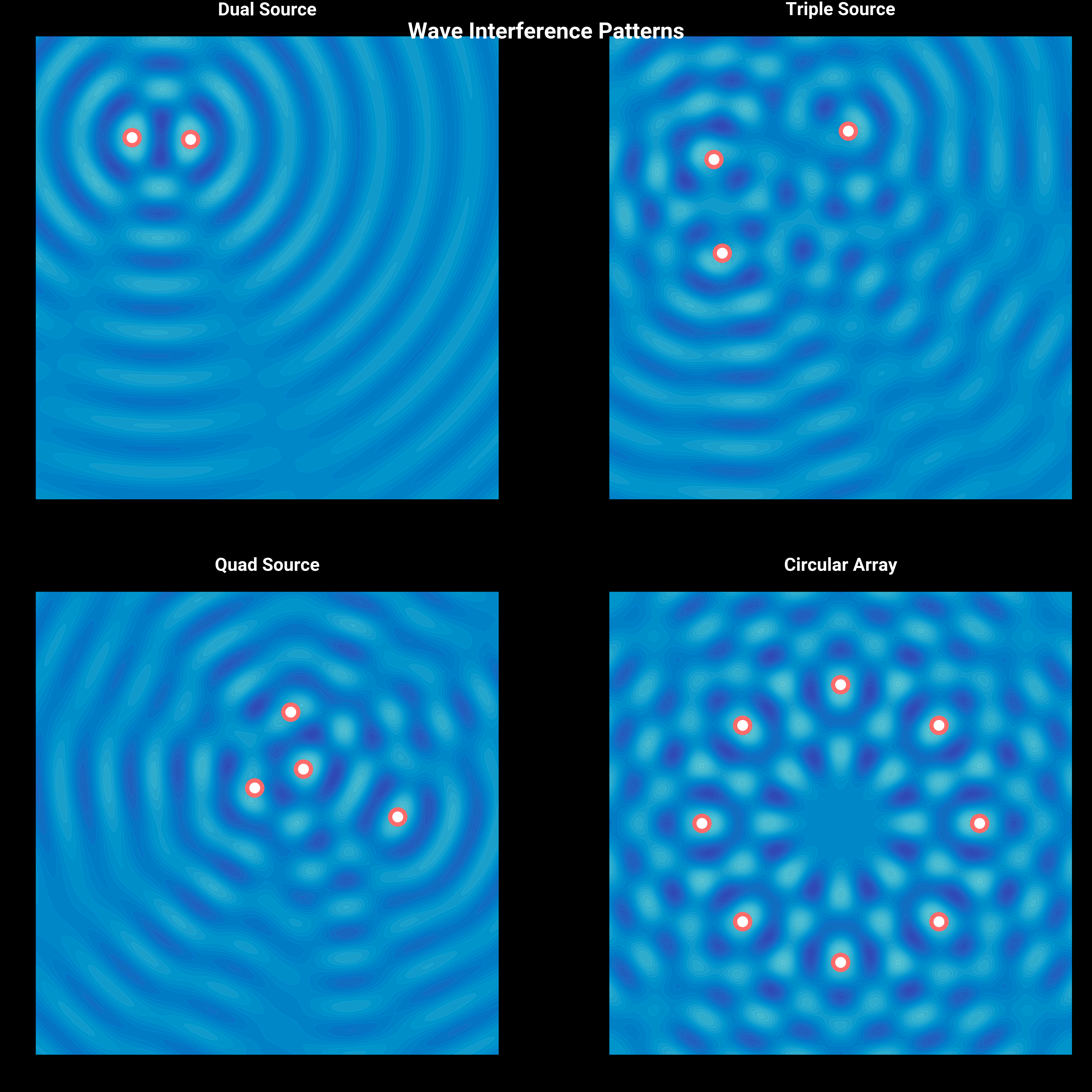
Sound Wave Interference Patterns

Visualize the beautiful patterns created by wave interference.

fig, axes = plt.subplots(2, 2, figsize=(dm.cm2in(18), dm.cm2in(18)))

x = np.linspace(-5, 5, 500)
y = np.linspace(-5, 5, 500)
X, Y = np.meshgrid(x, y)

patterns = [
    ("Dual Source", 2),
    ("Triple Source", 3),
    ("Quad Source", 4),
    ("Circular Array", 8),
]

for ax, (name, n_sources) in zip(axes.flat, patterns, strict=False):
    # Generate source positions
    if name == "Circular Array":
        angles = np.linspace(0, 2 * np.pi, n_sources, endpoint=False)
        sources = [(3 * np.cos(a), 3 * np.sin(a)) for a in angles]
    else:
        sources = [
            (np.random.uniform(-3, 3), np.random.uniform(-3, 3))
            for _ in range(n_sources)
        ]

    # Calculate interference pattern
    Z = np.zeros_like(X)
    for sx, sy in sources:
        R = np.sqrt((X - sx) ** 2 + (Y - sy) ** 2)
        Z += np.sin(2 * np.pi * R) / (1 + 0.5 * R)

    # Normalize
    Z = (Z - Z.min()) / (Z.max() - Z.min())

    # Create custom colormap
    colors_wave = dm.cspace("oc.indigo9", "oc.cyan3", n=256, space="oklch")
    wave_cmap = LinearSegmentedColormap.from_list(
        "wave", [c.to_hex() for c in colors_wave]
    )

    # Plot interference pattern
    im = ax.contourf(X, Y, Z, levels=20, cmap=wave_cmap, alpha=0.9)

    # Add source points
    for sx, sy in sources:
        ax.scatter(
            sx,
            sy,
            s=50,
            c="white",
            edgecolors="oc.red5",
            linewidths=2,
            zorder=10,
        )

    # Styling
    ax.set_xlim(-5, 5)
    ax.set_ylim(-5, 5)
    ax.set_aspect("equal")
    dm.hide_all_spines(ax)
    ax.set_title(name, fontsize=dm.fs(1), color="white", pad=10)
    ax.set_facecolor("black")

fig.suptitle(
    "Wave Interference Patterns",
    fontsize=dm.fs(3),
    color="white",
    weight="bold",
)
fig.patch.set_facecolor("black")

dm.simple_layout(fig)

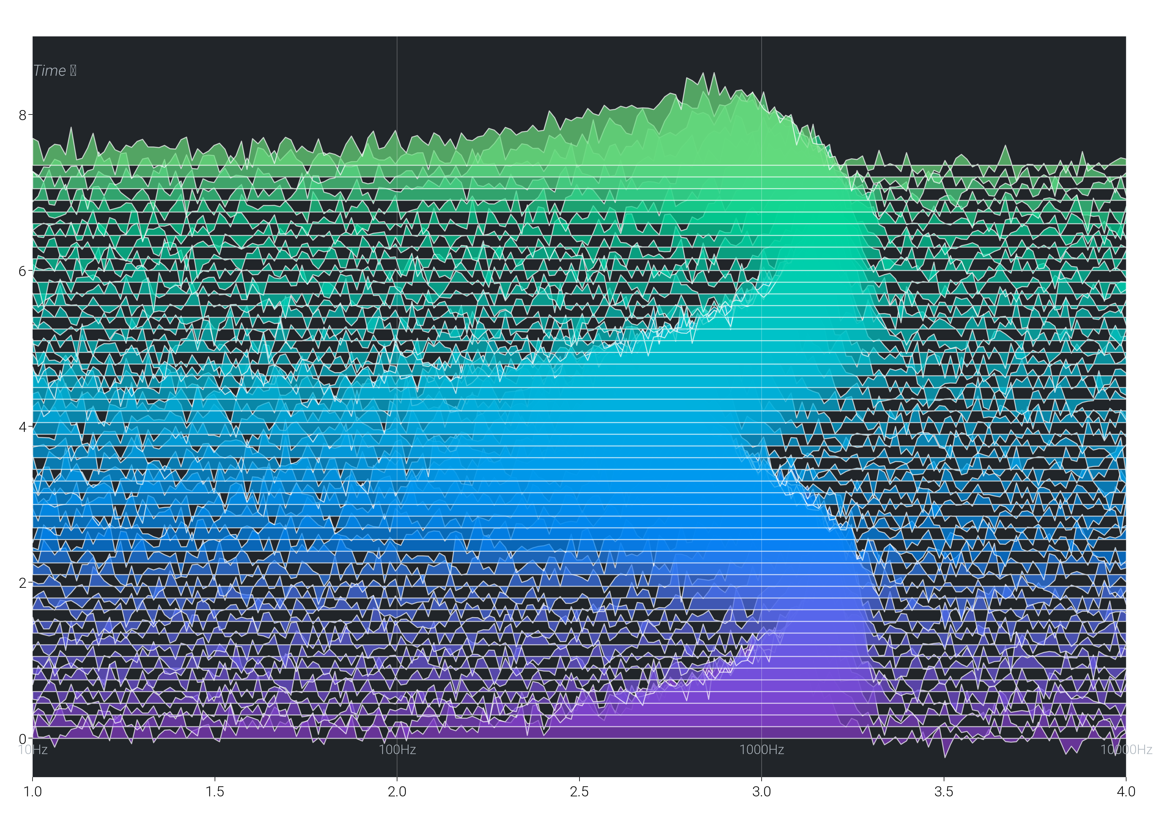
Frequency Response Waterfall

Create a 3D-like waterfall plot showing frequency response over time.

fig, ax = plt.subplots(figsize=(dm.cm2in(20), dm.cm2in(14)))

# Generate frequency response data
n_time_steps = 50
n_frequencies = 200
time = np.linspace(0, 10, n_time_steps)
freq = np.logspace(1, 4, n_frequencies)  # 10Hz to 10kHz

# Create varying frequency response
responses = []
for t in time:
    # Simulate changing filter response
    center_freq = 1000 * (1 + 0.5 * np.sin(t))
    bandwidth = 500 * (1 + 0.3 * np.cos(2 * t))
    response = np.exp(-(((freq - center_freq) / bandwidth) ** 2))
    response += 0.1 * np.random.randn(n_frequencies)  # Add noise
    responses.append(response)

# Plot waterfall
for i, (_t, response) in enumerate(zip(time, responses, strict=False)):
    # Create color based on time
    color = dm.cspace("oc.purple8", "oc.green4", n=n_time_steps)[i]

    # Offset for 3D effect
    y_offset = i * 0.15

    # Plot with fill
    ax.fill_between(
        np.log10(freq),
        y_offset,
        response + y_offset,
        color=color.to_hex(),
        alpha=0.7,
        edgecolor="white",
        linewidth=0.5,
    )

# Add frequency grid
for f in [10, 100, 1000, 10000]:
    ax.axvline(np.log10(f), color="white", lw=0.3, alpha=0.3)
    ax.text(
        np.log10(f),
        -0.2,
        f"{f}Hz",
        ha="center",
        fontsize=dm.fs(-1),
        color="oc.gray5",
    )

# Styling
ax.set_xlim(1, 4)
ax.set_ylim(-0.5, n_time_steps * 0.15 + 1.5)
dm.hide_all_spines(ax)
ax.set_facecolor("oc.gray9")

# Labels
ax.text(
    2.5,
    n_time_steps * 0.15 + 1.8,
    "Frequency Response Evolution",
    ha="center",
    fontsize=dm.fs(3),
    color="white",
    weight="bold",
)
ax.text(
    1,
    n_time_steps * 0.15 + 1,
    "Time →",
    fontsize=dm.fs(0),
    color="oc.gray5",
    style="italic",
)

dm.simple_layout(fig)

plt.show()