Gradient Flow Field Visualization

This example creates a mesmerizing flow field visualization with gradient colors that demonstrates dartwork-mpl’s advanced color interpolation and styling capabilities.

import matplotlib.patheffects as path_effects
import matplotlib.pyplot as plt
import numpy as np
from matplotlib.colors import LinearSegmentedColormap

import dartwork_mpl as dm

# Set random seed for reproducibility
np.random.seed(42)

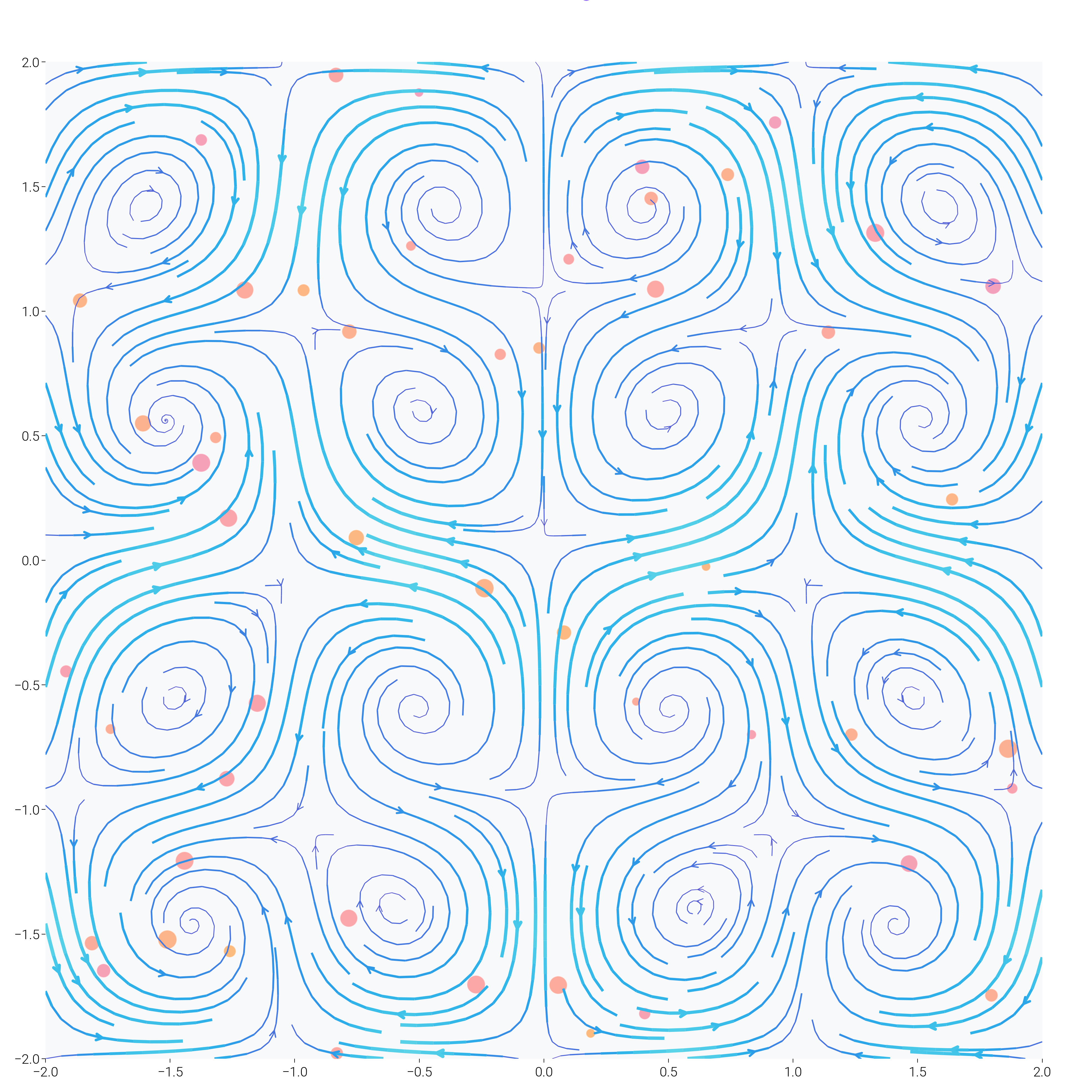
Organic Flow Field with Color Gradients

Create a flow field that looks like organic patterns with smooth color transitions.

dm.style.use("scientific")

# Create a grid of vectors
fig, ax = plt.subplots(figsize=(dm.cm2in(20), dm.cm2in(20)))

# Generate flow field
n_points = 25
x = np.linspace(-2, 2, n_points)
y = np.linspace(-2, 2, n_points)
X, Y = np.meshgrid(x, y)

# Create interesting flow patterns
t = 2.5
U = np.sin(np.pi * X) * np.cos(np.pi * Y) + 0.3 * np.sin(t * X)
V = -np.cos(np.pi * X) * np.sin(np.pi * Y) + 0.3 * np.cos(t * Y)

# Calculate magnitude for colors
M = np.sqrt(U**2 + V**2)

# Create custom colormap using dartwork's color interpolation
colors_flow = dm.cspace("oc.violet9", "oc.cyan3", n=256, space="oklch")
flow_cmap = LinearSegmentedColormap.from_list(
    "flow", [c.to_hex() for c in colors_flow]
)

# Plot streamlines with varying thickness
strm = ax.streamplot(
    X,
    Y,
    U,
    V,
    color=M,
    cmap=flow_cmap,
    linewidth=2 * M / M.max(),
    density=2,
    arrowsize=0.8,
    arrowstyle="->",
)

# Add particles flowing along the field
n_particles = 50
px = np.random.uniform(-2, 2, n_particles)
py = np.random.uniform(-2, 2, n_particles)
particle_colors = dm.cspace("oc.pink5", "oc.orange5", n=n_particles)

for _i, (x_p, y_p, color) in enumerate(zip(px, py, particle_colors, strict=False)):
    size = np.random.uniform(20, 100)
    ax.scatter(
        x_p,
        y_p,
        s=size,
        c=[color.to_hex()],
        alpha=0.6,
        edgecolors="white",
        linewidths=0.5,
    )

# Style the plot
dm.hide_all_spines(ax)
ax.set_xlim(-2, 2)
ax.set_ylim(-2, 2)
ax.set_aspect("equal")
ax.set_facecolor("oc.gray0")

# Add title with glow effect
title = ax.text(
    0,
    2.3,
    "Quantum Flow Dynamics",
    ha="center",
    va="center",
    fontsize=dm.fs(4),
    fontweight=dm.fw(3),
    color="white",
)
title.set_path_effects(
    [path_effects.withStroke(linewidth=3, foreground="oc.violet5")]
)

dm.simple_layout(fig)

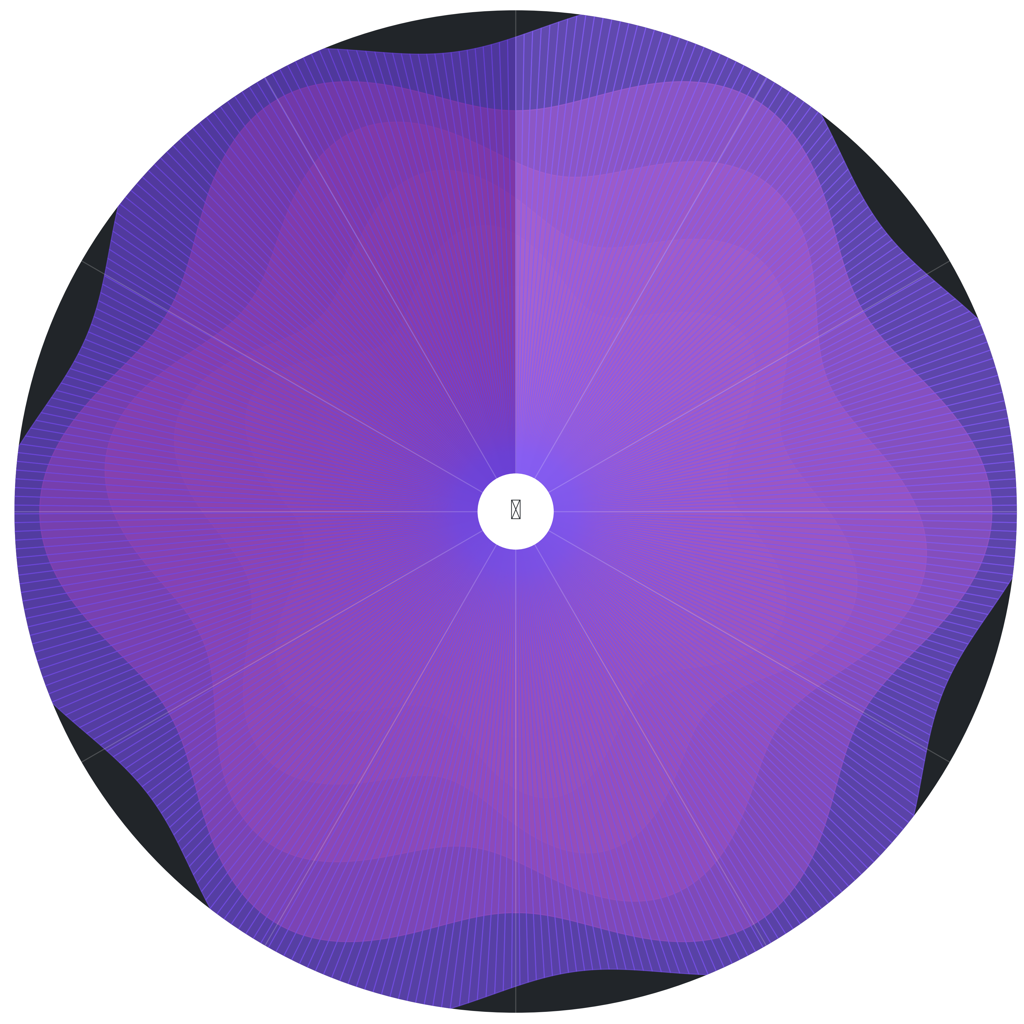
Radial Burst Pattern with Layered Gradients

Create a radial visualization that combines multiple gradient layers.

fig, ax = plt.subplots(
    figsize=(dm.cm2in(18), dm.cm2in(18)), subplot_kw={"projection": "polar"}
)

# Generate radial data
theta = np.linspace(0, 2 * np.pi, 360)
r_layers = 8

for layer in range(r_layers):
    # Create varying radius for each layer
    r_base = 0.5 + layer * 0.5
    r = r_base + 0.3 * np.sin(6 * theta + layer * np.pi / 4)

    # Color gradient for each layer
    layer_colors = dm.cspace(
        f"oc.{['blue', 'teal', 'green', 'yellow', 'orange', 'red', 'pink', 'violet'][layer]}5",
        f"oc.{['blue', 'teal', 'green', 'yellow', 'orange', 'red', 'pink', 'violet'][layer]}8",
        n=len(theta),
    )

    # Plot with transparency
    for i in range(len(theta) - 1):
        ax.fill_between(
            [theta[i], theta[i + 1]],
            0,
            [r[i], r[i + 1]],
            color=layer_colors[i].to_hex(),
            alpha=0.3 + 0.05 * layer,
        )

# Add radial spokes
for angle in np.linspace(0, 2 * np.pi, 12, endpoint=False):
    ax.plot([angle, angle], [0, 4], color="white", alpha=0.2, lw=0.5)

# Styling
ax.set_ylim(0, 4)
ax.set_theta_zero_location("N")
ax.set_theta_direction(-1)
dm.hide_all_spines(ax)
ax.set_xticks([])
ax.set_yticks([])
ax.set_facecolor("oc.gray9")

# Add center burst
center = plt.Circle(
    (0, 0), 0.3, transform=ax.transData._b, color="white", zorder=10
)
ax.add_patch(center)

ax.text(
    0,
    0,
    "✦",
    fontsize=dm.fs(6),
    ha="center",
    va="center",
    color="oc.gray9",
    weight="bold",
    zorder=11,
)

dm.simple_layout(fig)

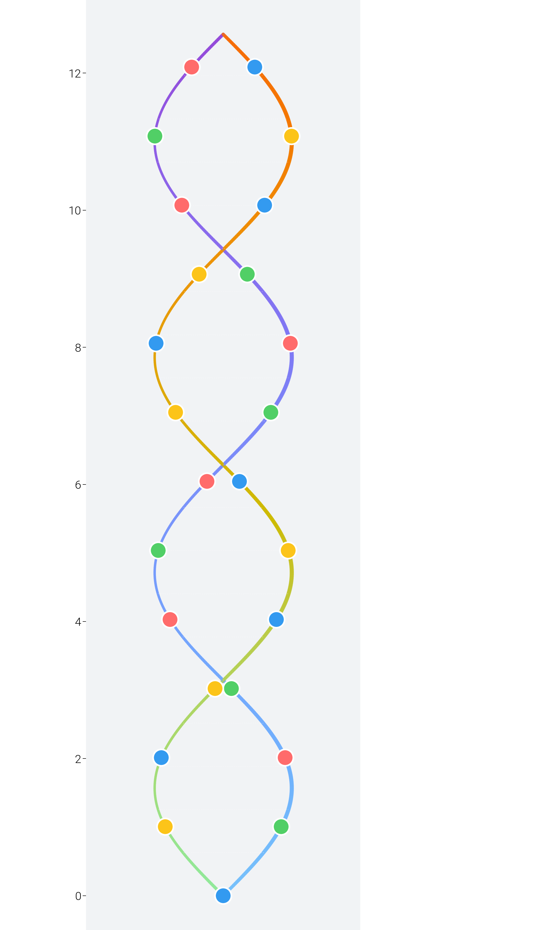
DNA Helix Visualization with Gradient Ribbons

Create a 3D-like DNA helix using creative 2D techniques.

fig, ax = plt.subplots(figsize=(dm.cm2in(12), dm.cm2in(20)))

# Generate helix coordinates
t = np.linspace(0, 4 * np.pi, 500)
x1 = np.sin(t)
x2 = np.sin(t + np.pi)
y = t

# Create gradient colors along the helix
colors_helix1 = dm.cspace("oc.blue3", "oc.purple7", n=len(t))
colors_helix2 = dm.cspace("oc.green3", "oc.orange7", n=len(t))

# Draw the helixes with varying width to create depth
for i in range(len(t) - 1):
    # First strand
    width1 = 2 + np.sin(t[i]) * 0.5  # Varying width for 3D effect
    ax.plot(
        [x1[i], x1[i + 1]],
        [y[i], y[i + 1]],
        color=colors_helix1[i].to_hex(),
        linewidth=width1,
        alpha=0.8,
        solid_capstyle="round",
    )

    # Second strand
    width2 = 2 - np.sin(t[i]) * 0.5
    ax.plot(
        [x2[i], x2[i + 1]],
        [y[i], y[i + 1]],
        color=colors_helix2[i].to_hex(),
        linewidth=width2,
        alpha=0.8,
        solid_capstyle="round",
    )

    # Connect strands at intervals
    if i % 25 == 0:
        ax.plot(
            [x1[i], x2[i]],
            [y[i], y[i]],
            color="white",
            alpha=0.3,
            lw=0.5,
            linestyle=":",
        )

# Add base pair representations
for i in range(0, len(t), 40):
    # Adenine-Thymine pairs
    if i % 80 == 0:
        ax.scatter(
            [x1[i], x2[i]],
            [y[i], y[i]],
            c=["oc.red5", "oc.blue5"],
            s=100,
            edgecolors="white",
            linewidths=1,
            zorder=5,
        )
    # Guanine-Cytosine pairs
    else:
        ax.scatter(
            [x1[i], x2[i]],
            [y[i], y[i]],
            c=["oc.green5", "oc.yellow5"],
            s=100,
            edgecolors="white",
            linewidths=1,
            zorder=5,
        )

# Styling
dm.hide_all_spines(ax)
ax.set_xlim(-2, 2)
ax.set_ylim(-0.5, 4 * np.pi + 0.5)
ax.set_aspect("equal")
ax.set_facecolor("oc.gray1")

# Add labels
ax.text(
    0,
    -1,
    "DNA Double Helix",
    ha="center",
    fontsize=dm.fs(3),
    color="white",
    weight="bold",
)
ax.text(
    0,
    4 * np.pi + 1,
    "A-T  G-C Base Pairs",
    ha="center",
    fontsize=dm.fs(0),
    color="oc.gray5",
)

dm.simple_layout(fig)

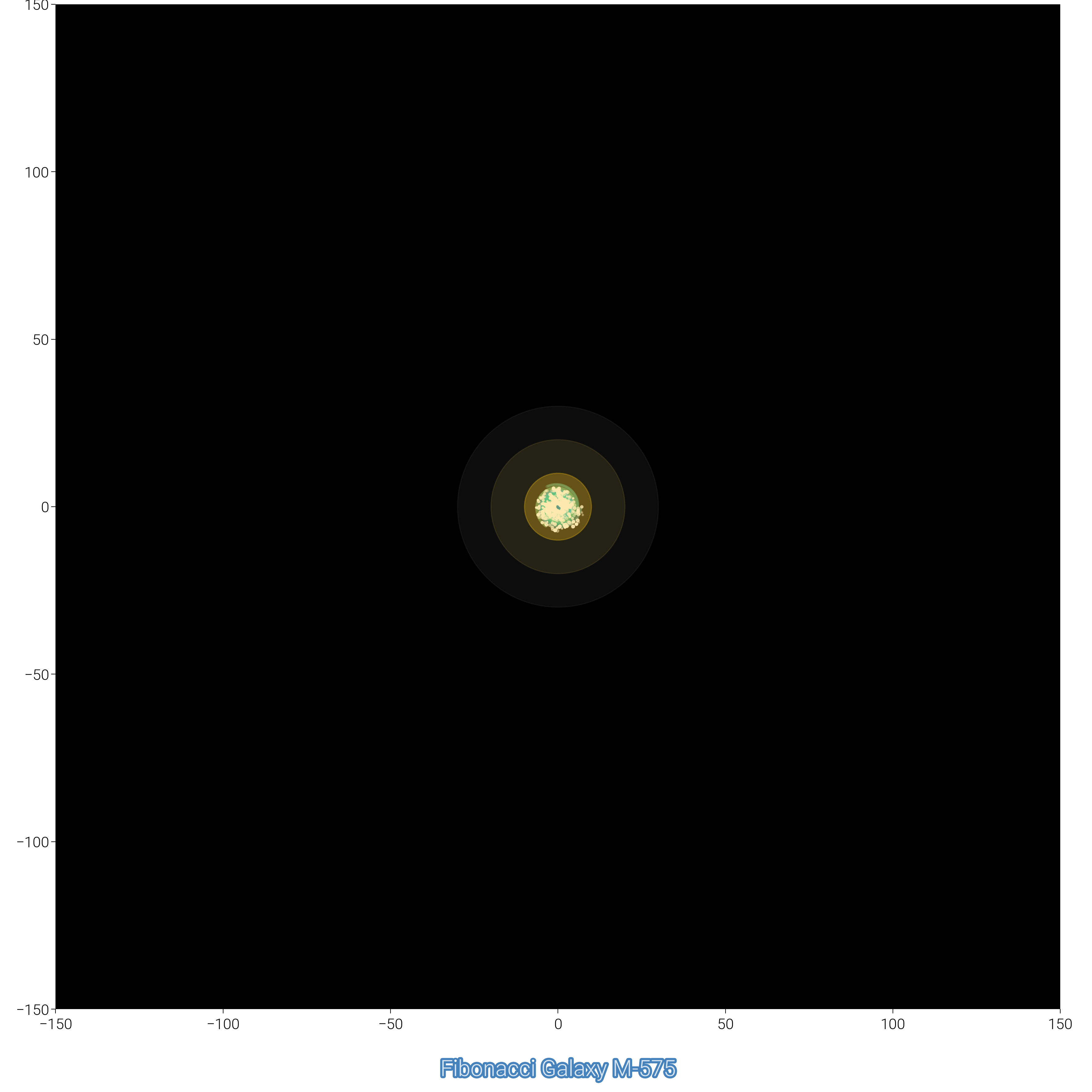
Fibonacci Spiral Galaxy

Create a galaxy visualization based on the Fibonacci spiral.

fig, ax = plt.subplots(figsize=(dm.cm2in(18), dm.cm2in(18)))


# Generate Fibonacci spiral
def fibonacci_spiral(n_points=1000):
    golden_ratio = (1 + np.sqrt(5)) / 2
    theta = np.linspace(0, 8 * np.pi, n_points)
    r = np.exp(theta / (2 * np.pi / np.log(golden_ratio)))
    x = r * np.cos(theta)
    y = r * np.sin(theta)
    return x, y, theta


x, y, theta = fibonacci_spiral(1500)

# Normalize for colors
norm_theta = (theta - theta.min()) / (theta.max() - theta.min())

# Create spiral galaxy effect with multiple arms
for arm in range(3):
    angle_offset = arm * 2 * np.pi / 3
    x_arm = x * np.cos(angle_offset) - y * np.sin(angle_offset)
    y_arm = x * np.sin(angle_offset) + y * np.cos(angle_offset)

    # Color gradient for each arm
    arm_colors = dm.cspace(
        f"oc.{['indigo', 'violet', 'blue'][arm]}9",
        f"oc.{['cyan', 'teal', 'green'][arm]}3",
        n=len(x),
    )

    # Draw arm with varying size points
    for i in range(0, len(x), 2):
        size = 0.5 + 20 * np.exp(-theta[i] / 10)
        alpha = 0.8 * np.exp(-theta[i] / 15)
        ax.scatter(
            x_arm[i],
            y_arm[i],
            s=size,
            c=[arm_colors[i].to_hex()],
            alpha=alpha,
            edgecolors="none",
        )

# Add star clusters
n_stars = 500
star_theta = np.random.uniform(0, 8 * np.pi, n_stars)
star_r = np.exp(star_theta / (2 * np.pi / np.log((1 + np.sqrt(5)) / 2)))
star_r *= np.random.uniform(0.8, 1.2, n_stars)  # Add randomness
star_x = star_r * np.cos(star_theta)
star_y = star_r * np.sin(star_theta)

ax.scatter(
    star_x,
    star_y,
    s=np.random.uniform(0.1, 2, n_stars),
    c="white",
    alpha=np.random.uniform(0.3, 1, n_stars),
)

# Add galaxy center
center_glow = plt.Circle((0, 0), 30, color="white", alpha=0.05)
ax.add_patch(center_glow)
center_glow2 = plt.Circle((0, 0), 20, color="oc.yellow3", alpha=0.1)
ax.add_patch(center_glow2)
center_core = plt.Circle((0, 0), 10, color="oc.yellow5", alpha=0.3)
ax.add_patch(center_core)

# Styling
dm.hide_all_spines(ax)
ax.set_xlim(-150, 150)
ax.set_ylim(-150, 150)
ax.set_aspect("equal")
ax.set_facecolor("black")

# Add title
title_text = ax.text(
    0,
    -170,
    "Fibonacci Galaxy M-" + str(np.random.randint(100, 999)),
    ha="center",
    fontsize=dm.fs(3),
    color="white",
    alpha=0.8,
)
title_text.set_path_effects(
    [path_effects.withStroke(linewidth=2, foreground="oc.blue9")]
)

dm.simple_layout(fig)

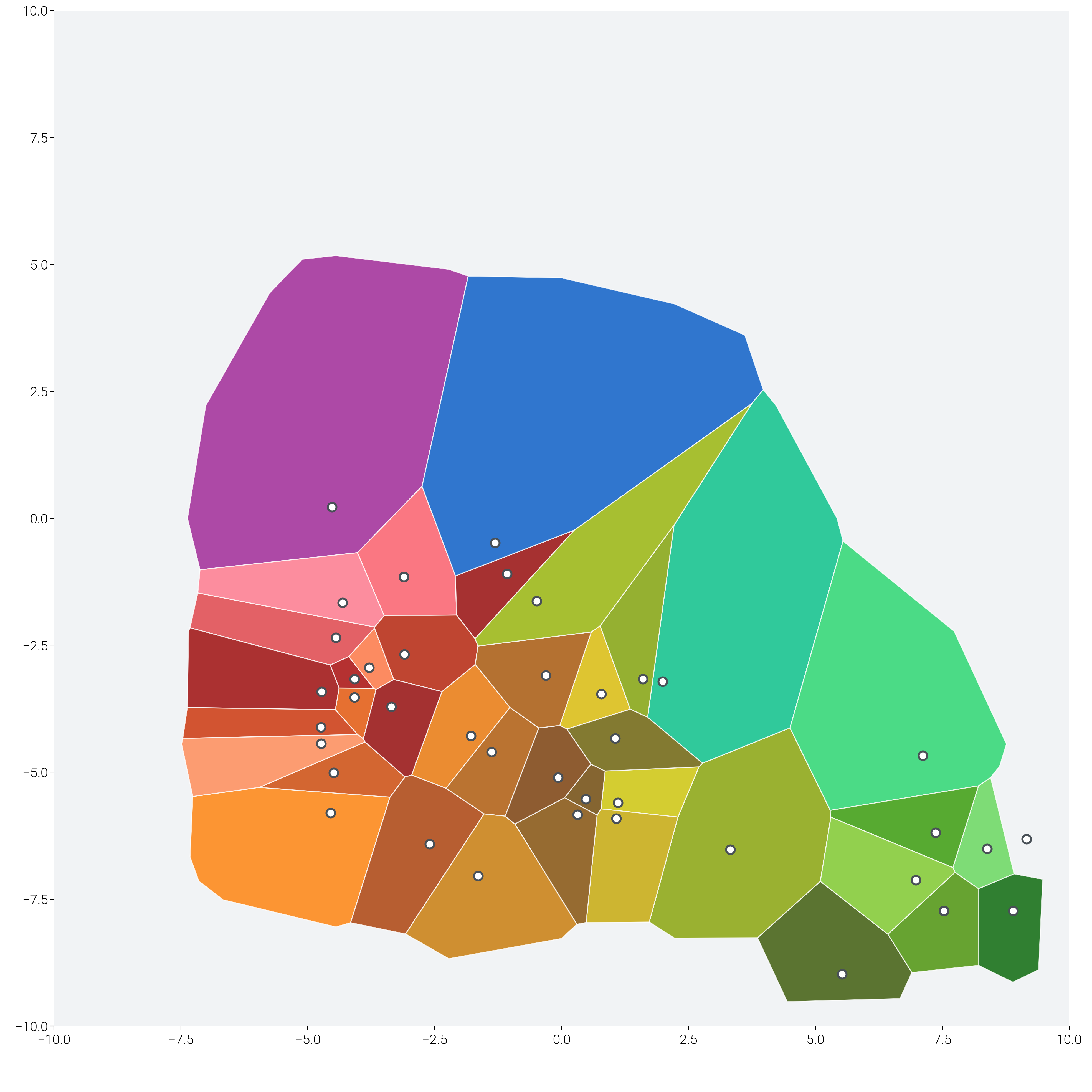
Generative Art: Voronoi Tessellation with Gradients

Create artistic Voronoi patterns with smooth color transitions.

from matplotlib.patches import Polygon  # noqa: E402
from scipy.spatial import Voronoi  # noqa: E402

fig, ax = plt.subplots(figsize=(dm.cm2in(20), dm.cm2in(20)))

# Generate random points with clustering
n_clusters = 5
n_points_per_cluster = 8
points = []

for _ in range(n_clusters):
    center_x = np.random.uniform(-8, 8)
    center_y = np.random.uniform(-8, 8)
    cluster_points = np.random.randn(n_points_per_cluster, 2) * 1.5 + [
        center_x,
        center_y,
    ]
    points.extend(cluster_points)

points = np.array(points)

# Add boundary points to ensure closed regions
boundary_points = []
for x in np.linspace(-10, 10, 10):
    boundary_points.append([x, -10])
    boundary_points.append([x, 10])
for y in np.linspace(-10, 10, 10):
    boundary_points.append([-10, y])
    boundary_points.append([10, y])

all_points = np.vstack([points, boundary_points])

# Compute Voronoi tessellation
vor = Voronoi(all_points)

# Color each region with gradient
for i, region in enumerate(vor.regions):
    if not region or -1 in region:
        continue

    polygon = [vor.vertices[j] for j in region]
    if len(polygon) > 2:
        # Check if polygon is within bounds
        polygon_array = np.array(polygon)
        if (
            polygon_array[:, 0].min() < -10
            or polygon_array[:, 0].max() > 10
            or polygon_array[:, 1].min() < -10
            or polygon_array[:, 1].max() > 10
        ):
            continue

        # Create color based on position and index
        center = polygon_array.mean(axis=0)
        hue = (np.arctan2(center[1], center[0]) + np.pi) / (2 * np.pi) * 360

        color = dm.oklch(0.6 + 0.2 * np.sin(i), 0.2, hue)

        poly = Polygon(
            polygon,
            facecolor=color.to_hex(),
            edgecolor="white",
            linewidth=0.5,
            alpha=0.8,
        )
        ax.add_patch(poly)

# Add decorative elements
for point in points[: n_clusters * n_points_per_cluster]:
    ax.scatter(
        *point, s=20, c="white", edgecolors="oc.gray7", linewidths=1, zorder=10
    )

# Styling
ax.set_xlim(-10, 10)
ax.set_ylim(-10, 10)
ax.set_aspect("equal")
dm.hide_all_spines(ax)
ax.set_facecolor("oc.gray1")

# Title
ax.text(
    0,
    -11,
    "Voronoi Dreams",
    ha="center",
    fontsize=dm.fs(3),
    color="white",
    weight="bold",
    alpha=0.9,
)

dm.simple_layout(fig)

plt.show()