Spine and Grid Customization

This example demonstrates various spine and grid utilities in dartwork-mpl, showing how to create different visual styles from minimal Tufte-inspired designs to fully framed publication figures.

import matplotlib.pyplot as plt
import numpy as np

import dartwork_mpl as dm

# Set up the data
np.random.seed(42)
x = np.linspace(0, 10, 100)
y1 = np.sin(x) + 0.1 * np.random.randn(100)
y2 = np.exp(-x / 5) * np.cos(2 * x)
y3 = x + 0.5 * np.random.randn(100)

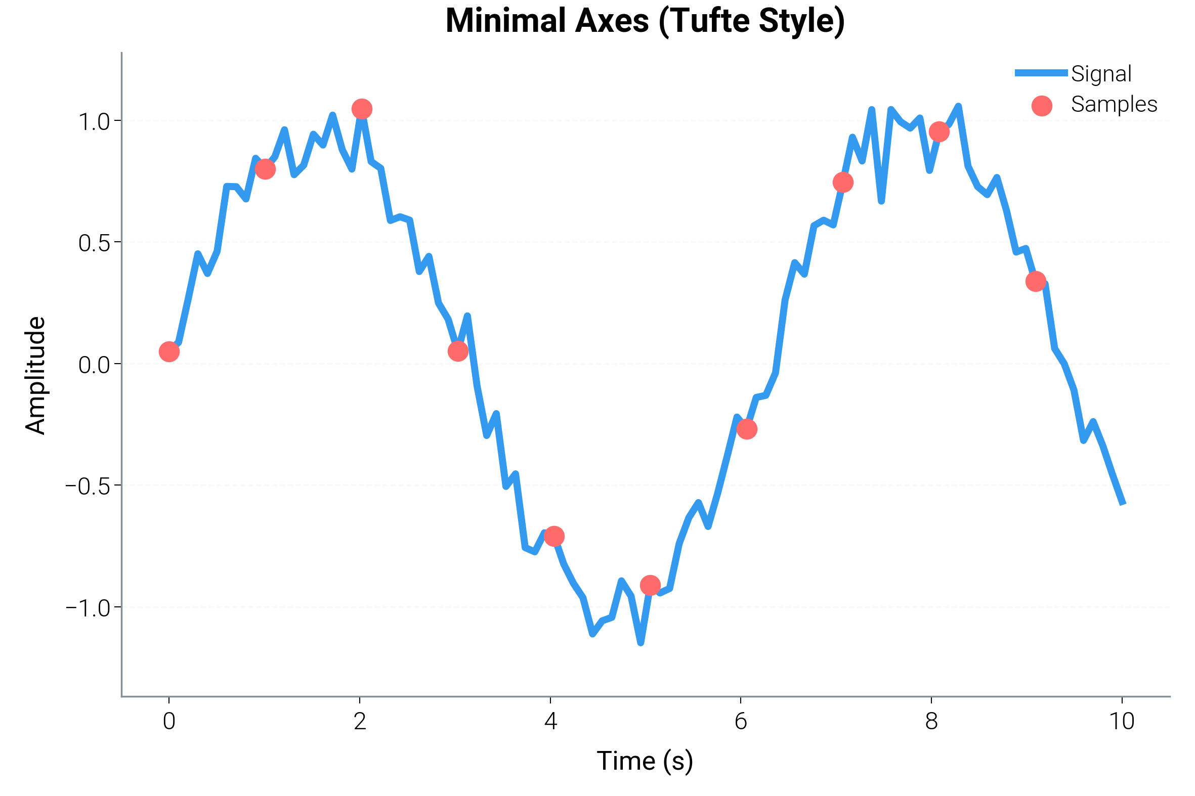
Minimal Axes (Tufte Style)

The most common pattern is creating clean, minimal axes that show only the essential spines (left and bottom).

dm.style.use("scientific")
fig, ax = plt.subplots(figsize=(dm.cm2in(12), dm.cm2in(8)))

ax.plot(x, y1, color="oc.blue5", lw=dm.lw(1), label="Signal")
ax.scatter(x[::10], y1[::10], color="oc.red5", s=30, zorder=5, label="Samples")

# Apply minimal style - keeps only left and bottom spines
dm.minimal_axes(ax)

ax.set_xlabel("Time (s)", fontsize=dm.fs(0))
ax.set_ylabel("Amplitude", fontsize=dm.fs(0))
ax.set_title("Minimal Axes (Tufte Style)", fontsize=dm.fs(2))
ax.legend(fontsize=dm.fs(-1), frameon=False)

dm.simple_layout(fig)

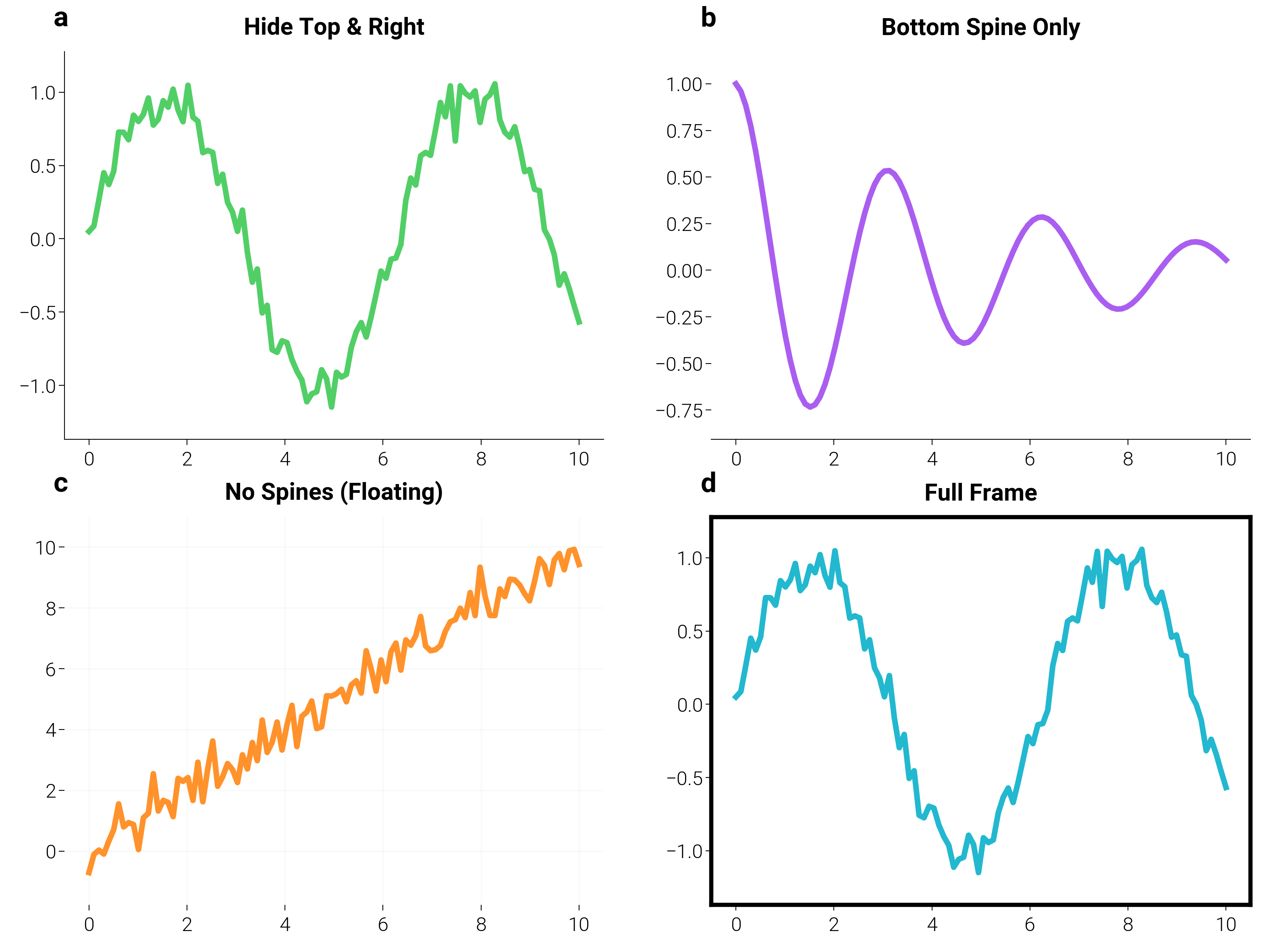
Custom Spine Visibility

Control exactly which spines are visible for different effects.

fig, axes = plt.subplots(2, 2, figsize=(dm.cm2in(16), dm.cm2in(12)))

# Top-left: Hide top and right (same as minimal_axes)
ax1 = axes[0, 0]
ax1.plot(x, y1, color="oc.green5", lw=dm.lw(1))
dm.hide_spines(ax1, ["top", "right"])
ax1.set_title("Hide Top & Right", fontsize=dm.fs(1))

# Top-right: Show only bottom spine
ax2 = axes[0, 1]
ax2.plot(x, y2, color="oc.purple5", lw=dm.lw(1))
dm.show_only_spines(ax2, ["bottom"])
ax2.set_title("Bottom Spine Only", fontsize=dm.fs(1))

# Bottom-left: Hide all spines (floating plot)
ax3 = axes[1, 0]
ax3.plot(x, y3, color="oc.orange5", lw=dm.lw(1))
dm.hide_all_spines(ax3)
dm.add_grid(ax3, alpha=0.2)  # Add grid for reference
ax3.set_title("No Spines (Floating)", fontsize=dm.fs(1))

# Bottom-right: Full frame
ax4 = axes[1, 1]
ax4.plot(x, y1, color="oc.cyan5", lw=dm.lw(1))
dm.add_frame(ax4, color="black", linewidth=1.5)
ax4.set_title("Full Frame", fontsize=dm.fs(1))

dm.label_axes(axes.flat)
dm.simple_layout(fig)

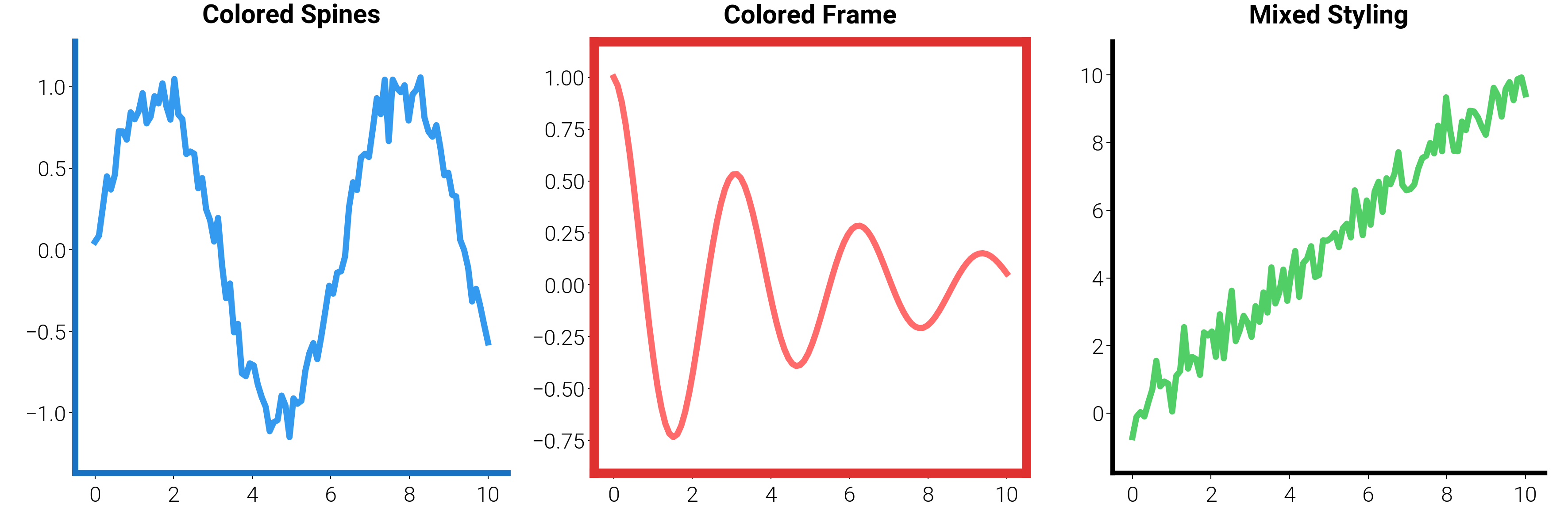
Spine Styling

Customize spine appearance with color and linewidth.

fig, axes = plt.subplots(1, 3, figsize=(dm.cm2in(18), dm.cm2in(6)))

# Left: Colored spines
ax1 = axes[0]
ax1.plot(x, y1, color="oc.blue5", lw=dm.lw(1))
dm.style_spines(ax1, color="oc.blue8", linewidth=2, which=["left", "bottom"])
dm.hide_spines(ax1, ["top", "right"])
ax1.set_title("Colored Spines", fontsize=dm.fs(1))

# Middle: Thick frame with color
ax2 = axes[1]
ax2.plot(x, y2, color="oc.red5", lw=dm.lw(1))
dm.add_frame(ax2, color="oc.red8", linewidth=3)
ax2.set_title("Colored Frame", fontsize=dm.fs(1))

# Right: Mixed styling
ax3 = axes[2]
ax3.plot(x, y3, color="oc.green5", lw=dm.lw(1))
dm.style_spines(ax3, color="gray", linewidth=0.5, which=["top", "right"])
dm.style_spines(ax3, color="black", linewidth=1.5, which=["left", "bottom"])
ax3.set_title("Mixed Styling", fontsize=dm.fs(1))

dm.simple_layout(fig)

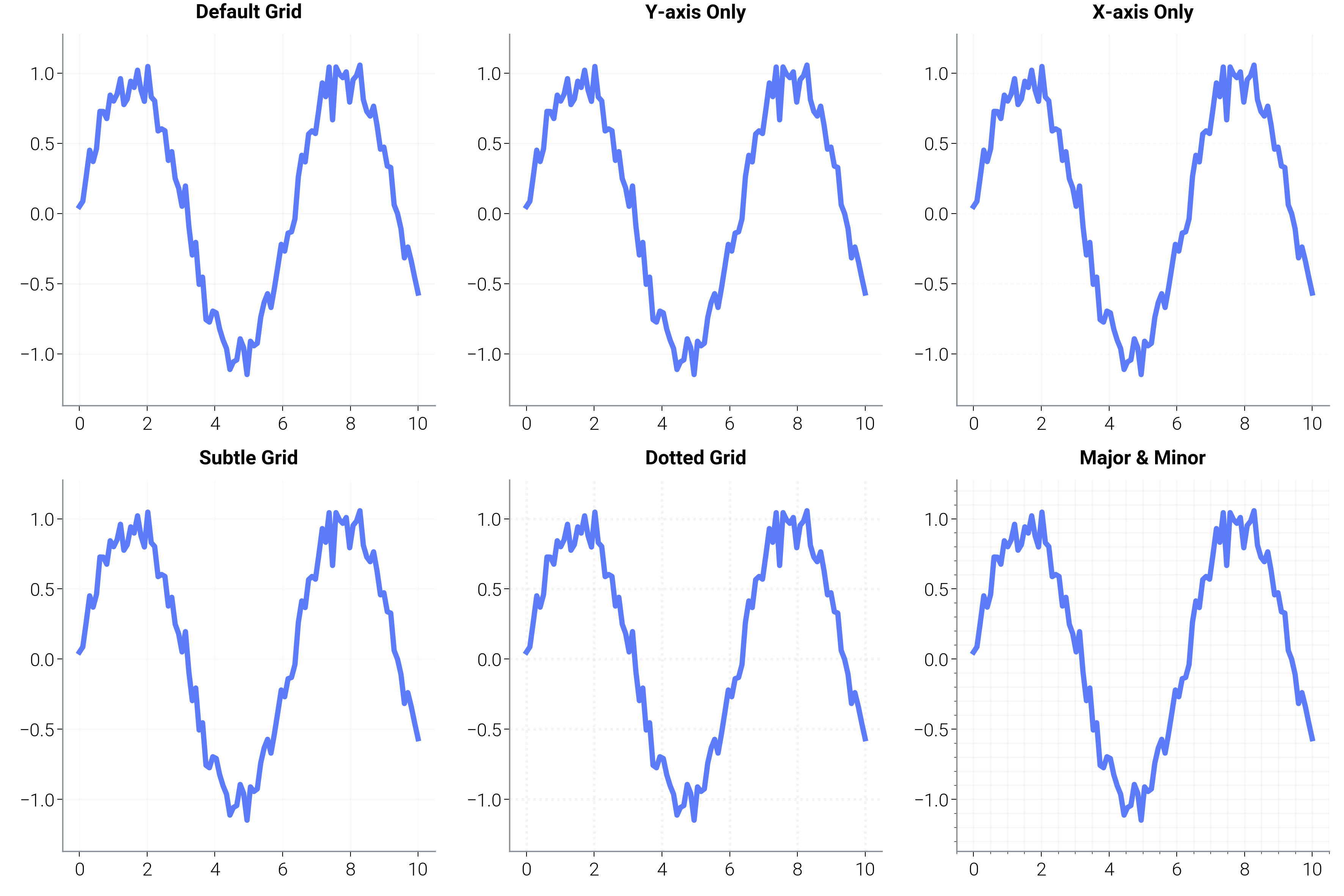
Grid Customization

Add and style grids for better readability.

fig, axes = plt.subplots(2, 3, figsize=(dm.cm2in(18), dm.cm2in(12)))

# Different grid styles
grid_configs = [
    {"title": "Default Grid", "kwargs": {}},
    {"title": "Y-axis Only", "kwargs": {"axis": "y"}},
    {"title": "X-axis Only", "kwargs": {"axis": "x"}},
    {
        "title": "Subtle Grid",
        "kwargs": {"alpha": 0.2, "linestyle": "-", "linewidth": 0.5},
    },
    {
        "title": "Dotted Grid",
        "kwargs": {"alpha": 0.4, "linestyle": ":", "linewidth": 1},
    },
    {"title": "Major & Minor", "kwargs": {"which": "both", "alpha": 0.3}},
]

for ax, config in zip(axes.flat, grid_configs, strict=False):
    ax.plot(x, y1, color="oc.indigo5", lw=dm.lw(1))
    dm.minimal_axes(ax)
    dm.add_grid(ax, **config["kwargs"])
    ax.set_title(config["title"], fontsize=dm.fs(0))

    # Add minor ticks for the last example
    if config["title"] == "Major & Minor":
        ax.minorticks_on()

dm.simple_layout(fig)

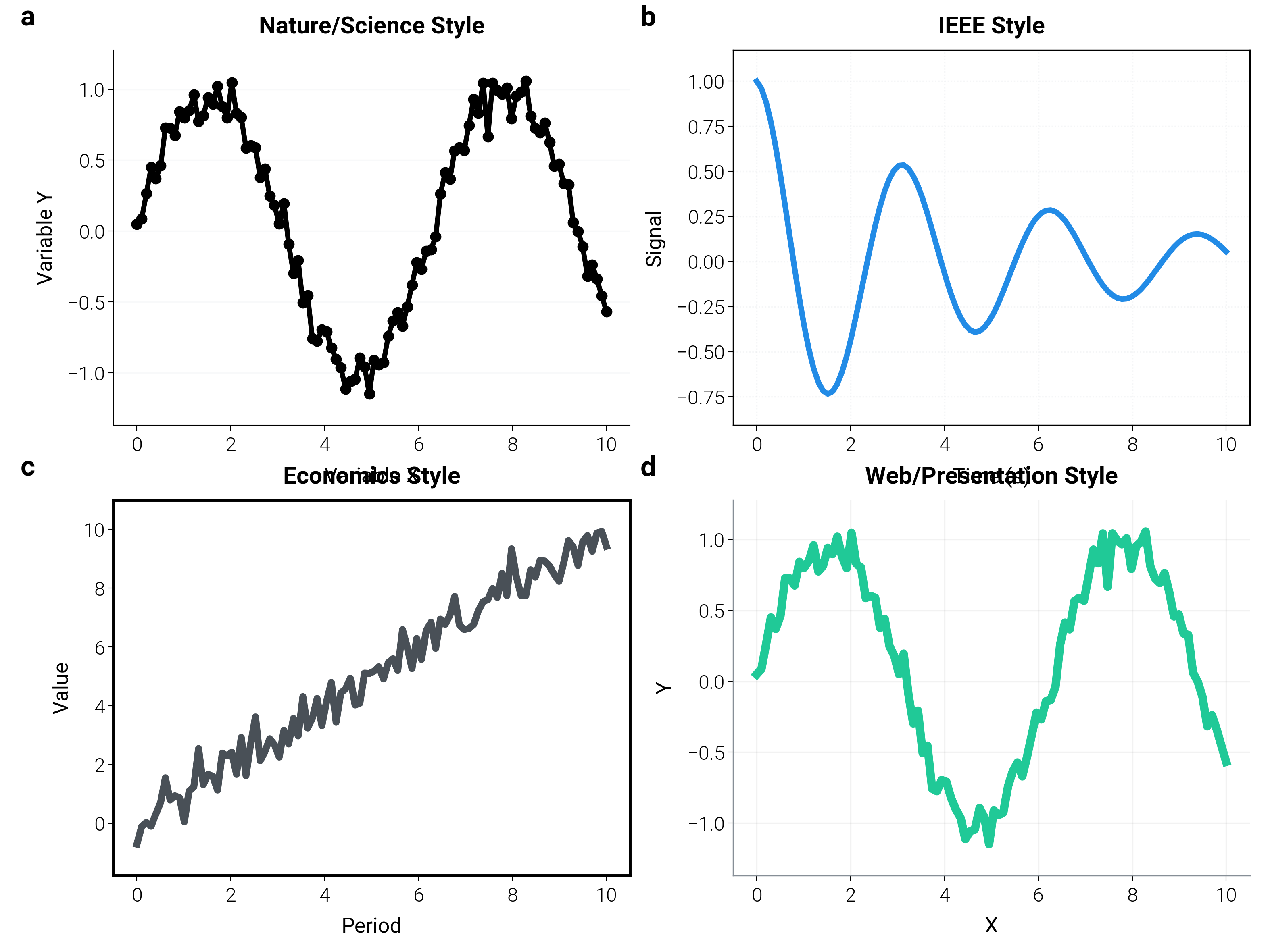
Publication Styles

Different journals and venues have different preferences. Here are common patterns for various publication types.

fig, axes = plt.subplots(2, 2, figsize=(dm.cm2in(16), dm.cm2in(12)))

# Nature/Science style
ax1 = axes[0, 0]
ax1.plot(x, y1, "o-", color="black", markersize=3, lw=dm.lw(0.8))
dm.hide_spines(ax1, ["top", "right"])
dm.add_grid(ax1, alpha=0.2, axis="y", linestyle="-")
ax1.set_title("Nature/Science Style", fontsize=dm.fs(1))
ax1.set_xlabel("Variable X", fontsize=dm.fs(0))
ax1.set_ylabel("Variable Y", fontsize=dm.fs(0))

# IEEE style
ax2 = axes[0, 1]
ax2.plot(x, y2, color="oc.blue6", lw=dm.lw(1))
dm.add_frame(ax2, color="black", linewidth=0.5)
dm.add_grid(ax2, which="major", alpha=0.3, linestyle=":")
ax2.set_title("IEEE Style", fontsize=dm.fs(1))
ax2.set_xlabel("Time (s)", fontsize=dm.fs(0))
ax2.set_ylabel("Signal", fontsize=dm.fs(0))

# Economics journals
ax3 = axes[1, 0]
ax3.plot(x, y3, color="oc.gray7", lw=dm.lw(1.5))
dm.add_frame(ax3, color="black", linewidth=1)
# No grid for clean look
ax3.set_title("Economics Style", fontsize=dm.fs(1))
ax3.set_xlabel("Period", fontsize=dm.fs(0))
ax3.set_ylabel("Value", fontsize=dm.fs(0))

# Web/Presentation
ax4 = axes[1, 1]
ax4.plot(x, y1, color="oc.teal5", lw=dm.lw(2))
dm.minimal_axes(ax4)
dm.add_grid(ax4, alpha=0.1, linestyle="-", color="gray")
ax4.set_title("Web/Presentation Style", fontsize=dm.fs(1))
ax4.set_xlabel("X", fontsize=dm.fs(0))
ax4.set_ylabel("Y", fontsize=dm.fs(0))

dm.label_axes(axes.flat)
dm.simple_layout(fig)

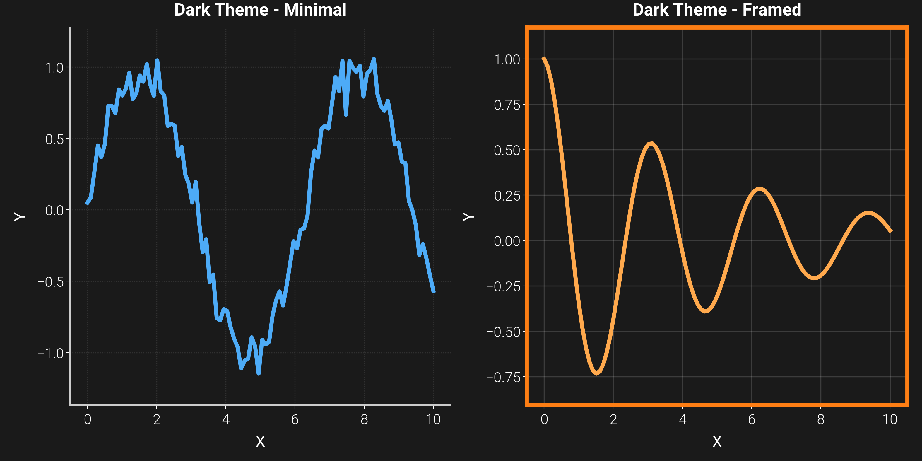
Dark Theme Support

Spine utilities work seamlessly with dark themes.

dm.style.use("dark")
dm.style.use("scientific")
fig, (ax1, ax2) = plt.subplots(
    1, 2, figsize=(dm.cm2in(16), dm.cm2in(8)), facecolor="#1a1a1a"
)

# Left: Minimal with light spines
ax1.plot(x, y1, color="oc.blue4", lw=dm.lw(1))
dm.minimal_axes(ax1)
dm.style_spines(ax1, color="#CCCCCC", linewidth=0.8)
dm.add_grid(ax1, alpha=0.1, color="white", linestyle=":")
ax1.set_title("Dark Theme - Minimal", fontsize=dm.fs(1), color="white")
ax1.set_xlabel("X", fontsize=dm.fs(0), color="white")
ax1.set_ylabel("Y", fontsize=dm.fs(0), color="white")
ax1.tick_params(colors="white")
ax1.set_facecolor("#1a1a1a")

# Right: Framed with colored border
ax2.plot(x, y2, color="oc.orange4", lw=dm.lw(1))
dm.add_frame(ax2, color="oc.orange6", linewidth=2)
dm.add_grid(ax2, alpha=0.15, color="white", linestyle="-", linewidth=0.5)
ax2.set_title("Dark Theme - Framed", fontsize=dm.fs(1), color="white")
ax2.set_xlabel("X", fontsize=dm.fs(0), color="white")
ax2.set_ylabel("Y", fontsize=dm.fs(0), color="white")
ax2.tick_params(colors="white")
ax2.set_facecolor("#1a1a1a")

dm.simple_layout(fig)

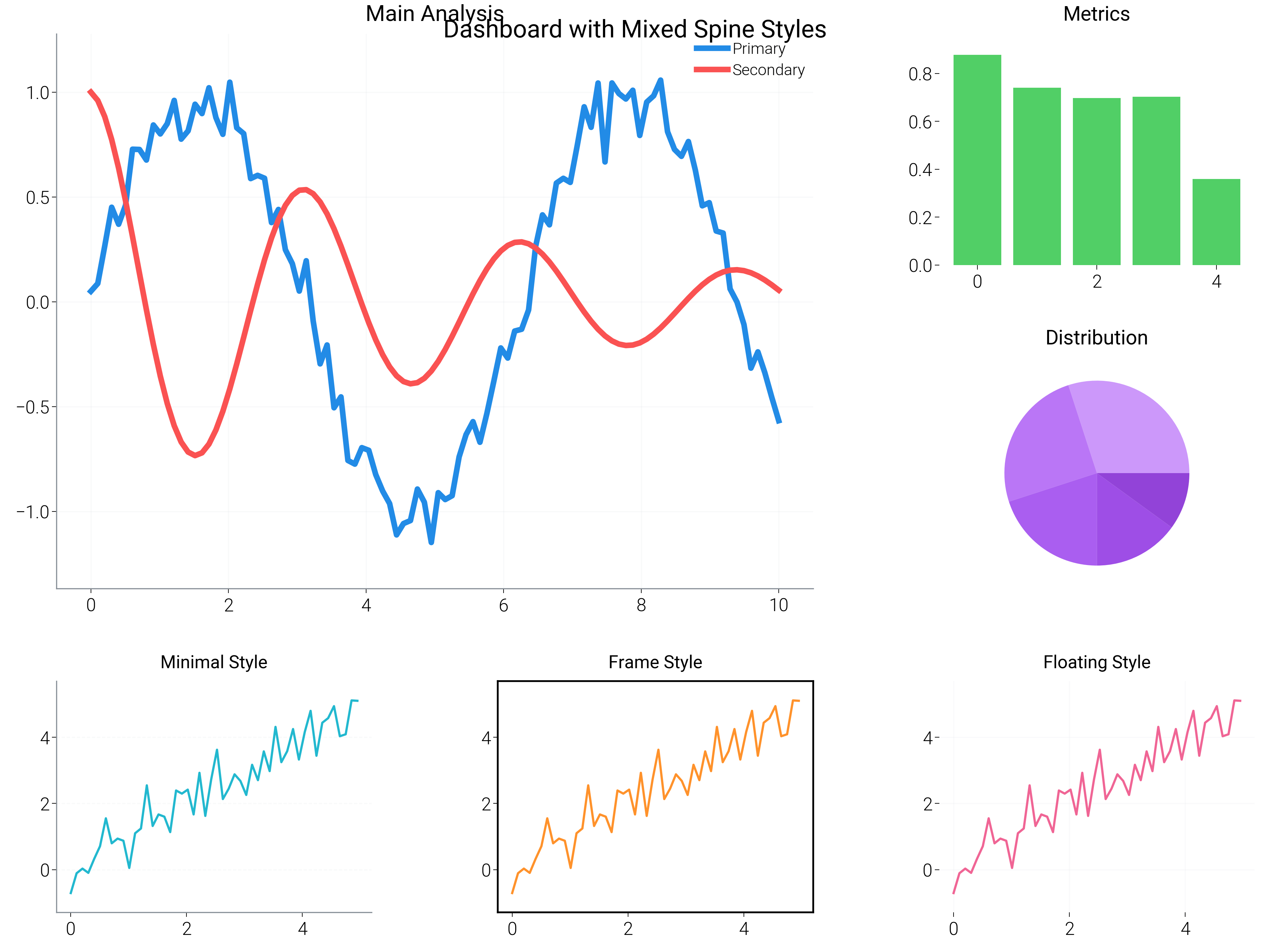
Complete Dashboard Example

Combining different spine styles in a multi-panel figure.

dm.style.use("report")  # Switch back to light theme
fig = plt.figure(figsize=(dm.cm2in(20), dm.cm2in(15)))
gs = fig.add_gridspec(3, 3, hspace=0.4, wspace=0.4)

# Main plot (2x2 in top-left)
ax_main = fig.add_subplot(gs[:2, :2])
ax_main.plot(x, y1, color="oc.blue6", lw=dm.lw(1.5), label="Primary")
ax_main.plot(x, y2, color="oc.red6", lw=dm.lw(1.5), label="Secondary")
dm.minimal_axes(ax_main)
dm.add_grid(ax_main, alpha=0.2)
ax_main.set_title("Main Analysis", fontsize=dm.fs(2))
ax_main.legend(fontsize=dm.fs(-1))

# Top-right panel
ax_tr = fig.add_subplot(gs[0, 2])
ax_tr.bar(range(5), np.random.rand(5), color="oc.green5")
dm.hide_all_spines(ax_tr)
ax_tr.set_title("Metrics", fontsize=dm.fs(1))

# Middle-right panel
ax_mr = fig.add_subplot(gs[1, 2])
ax_mr.pie([30, 25, 20, 15, 10], colors=[f"oc.purple{i}" for i in range(3, 8)])
ax_mr.set_title("Distribution", fontsize=dm.fs(1))

# Bottom row - three panels with different styles
for i, style in enumerate(["minimal", "frame", "floating"]):
    ax = fig.add_subplot(gs[2, i])
    ax.plot(x[:50], y3[:50], color=f"oc.{['cyan', 'orange', 'pink'][i]}5")

    if style == "minimal":
        dm.minimal_axes(ax)
    elif style == "frame":
        dm.add_frame(ax, color="black", linewidth=0.8)
    else:  # floating
        dm.hide_all_spines(ax)
        dm.add_grid(ax, alpha=0.15)

    ax.set_title(f"{style.capitalize()} Style", fontsize=dm.fs(0))

plt.suptitle("Dashboard with Mixed Spine Styles", fontsize=dm.fs(3), y=0.98)
dm.simple_layout(fig)

plt.show()