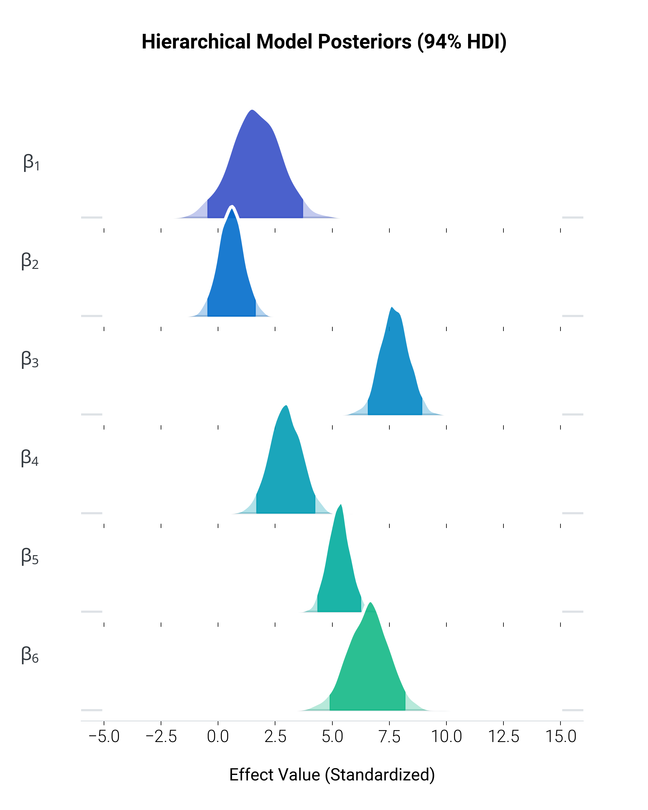
Bayesian MCMC Posterior Ridgelines

Visualizing the posterior distributions of multiple parameters sampled via Markov Chain Monte Carlo (MCMC). This “joyplot” or ridgeline plot effectively compares parameter uncertainties.

In Bayesian workflows, it’s customary to highlight the Highest Density Interval (HDI). Here, we overlay a global cspace gradient across the parameters, shading the bulk of the distributions to give depth and immediate visual separation.

import matplotlib.pyplot as plt
import numpy as np
from scipy.stats import gaussian_kde

import dartwork_mpl as dm

dm.style.use("report")

# Generate synthetic MCMC trace data for 6 parameters
np.random.seed(101)
parameters = [f"$\\beta_{i}$" for i in range(1, 7)]
n_params = len(parameters)

traces = []
for i in range(n_params):
    mean = np.random.uniform(-2, 5) + (i * 1.5)
    std = np.random.uniform(0.5, 1.5)
    traces.append(np.random.normal(mean, std, 3000))

# Colors extracted from an OKLCH perceptual space
c1 = dm.named("oc.indigo9").to_hex()
c2 = dm.named("oc.teal6").to_hex()
ridge_colors = dm.cspace(c1, c2, n=n_params, space="oklch")

fig, axes = plt.subplots(
    n_params, 1, figsize=(dm.SW * 1.2, dm.SW * 1.5), sharex=True
)
fig.subplots_adjust(
    hspace=-0.25
)  # Negative hspace for the overlapping ridgeline effect

x_eval = np.linspace(-5, 15, 300)

for _i, (ax, trace, color, label) in enumerate(
    zip(axes, traces, ridge_colors, parameters, strict=False)
):
    kde = gaussian_kde(trace)
    density = kde(x_eval)

    # Scale density for uniform visual height in the overlap
    density_scaled = density / density.max()

    # Extract the 94% HDI
    lo = np.percentile(trace, 3)
    hi = np.percentile(trace, 97)

    # White outline
    ax.plot(x_eval, density_scaled, color="white", lw=1.5, zorder=5)

    # Fill the entire distribution lightly
    ax.fill_between(
        x_eval, 0, density_scaled, color=color.to_hex(), alpha=0.3, zorder=4
    )

    # Fill the HDI bounds heavily
    hdi_mask = (x_eval >= lo) & (x_eval <= hi)
    ax.fill_between(
        x_eval,
        0,
        density_scaled,
        where=hdi_mask,
        color=color.to_hex(),
        alpha=0.85,
        zorder=4,
    )

    # Cleanup individual axes
    for spine in ax.spines.values():
        spine.set_visible(False)
    ax.set_yticks([])
    ax.set_ylabel(
        label,
        rotation=0,
        labelpad=20,
        ha="right",
        va="center",
        fontsize=dm.fs(0.5),
        weight="bold",
        color="oc.gray8",
    )
    ax.patch.set_alpha(0)  # Transparent background

    ax.axhline(0, color="oc.gray3", lw=1, zorder=3)

# Shared x-axis on the bottom
axes[-1].spines["bottom"].set_visible(True)
axes[-1].spines["bottom"].set_color("oc.gray4")
axes[-1].set_xlabel(
    "Effect Value (Standardized)", fontsize=dm.fs(0), labelpad=10
)

fig.suptitle(
    "Hierarchical Model Posteriors (94% HDI)",
    fontsize=dm.fs(1.5),
    weight="bold",
    y=0.96,
)