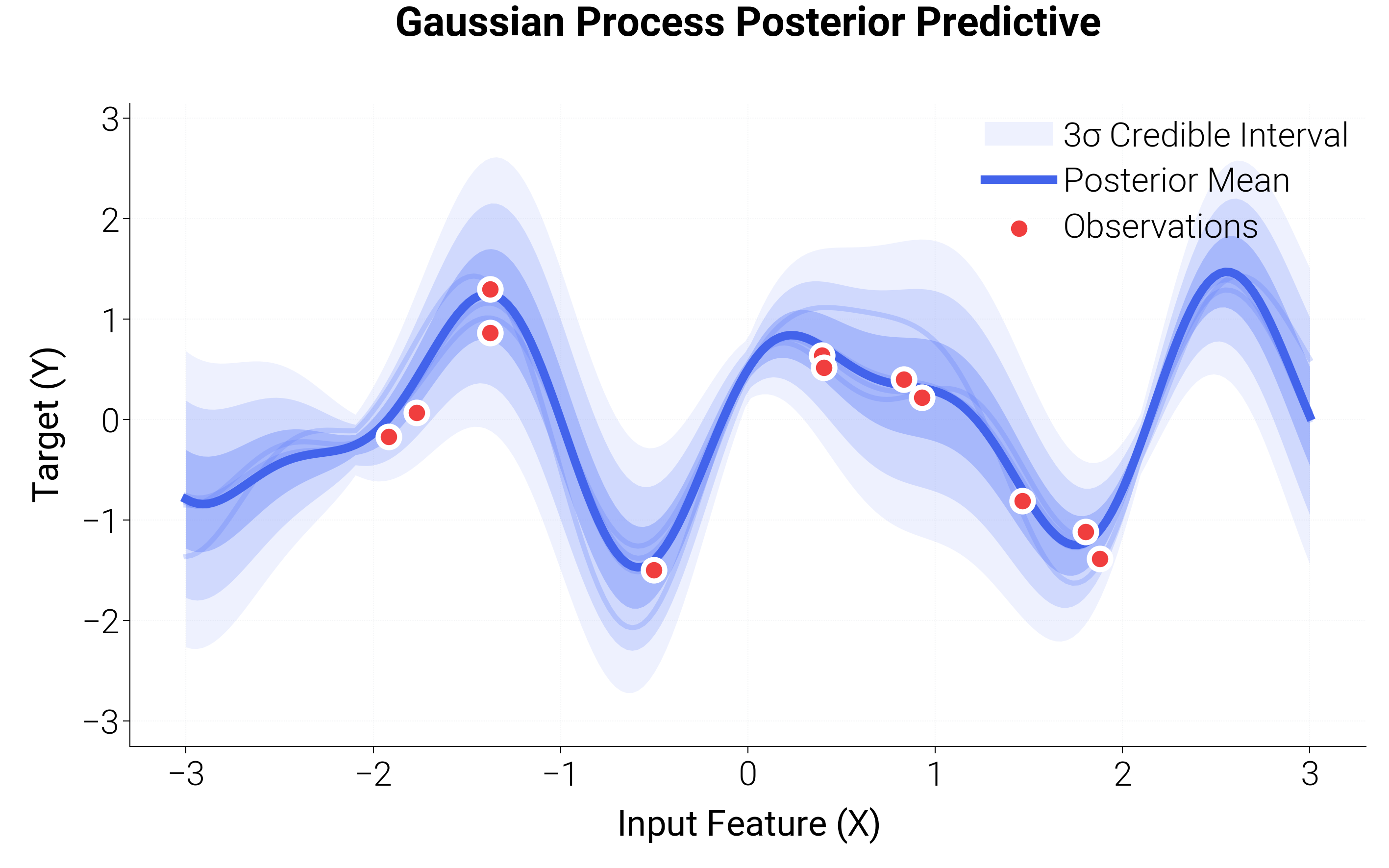
Gaussian Process Regression

A quintessential Bayesian machine learning visualization showing predictive uncertainty. This plot visualizes the GP predictive mean, individual sample functions drawn from the posterior, and beautifully shaded gradient bands representing 1σ, 2σ, and 3σ credible intervals.

import matplotlib.pyplot as plt
import numpy as np

import dartwork_mpl as dm

dm.style.use("presentation")

np.random.seed(42)


def true_fn(x):
    return np.sin(3 * x) + 0.5 * np.cos(5 * x)


# Observations
x_train = np.random.uniform(-2, 2, 12)
y_train = true_fn(x_train) + np.random.normal(0, 0.2, len(x_train))

x_test = np.linspace(-3, 3, 200)

# Simulate a GP posterior predictive
mean_pred = true_fn(x_test)
std_pred = 0.1 + 0.4 * np.abs(np.sin(x_test * 1.5))

fig, ax = plt.subplots(figsize=(dm.SW * 1.6, dm.SW * 1.0))

# 1. Plot the uncertainty bands (1σ, 2σ, 3σ)
base_color = dm.named("oc.indigo5")

for sigma, alpha in [(3, 0.1), (2, 0.2), (1, 0.35)]:
    ax.fill_between(
        x_test,
        mean_pred - sigma * std_pred,
        mean_pred + sigma * std_pred,
        color=base_color.to_hex(),
        alpha=alpha,
        lw=0,
        label=f"{sigma}σ Credible Interval" if sigma == 3 else "",
    )

# 2. Draw sample functions from the posterior
for _i in range(4):
    sample_path = mean_pred + np.random.normal(0, 1) * std_pred * np.sin(
        x_test * np.random.uniform(2, 4)
    )
    ax.plot(
        x_test,
        sample_path,
        color=base_color.to_hex(),
        alpha=0.25,
        lw=dm.lw(0.5),
    )

# 3. Plot predictive mean
ax.plot(
    x_test, mean_pred, color="oc.indigo7", lw=dm.lw(1.5), label="Posterior Mean"
)

# 4. Plot training observations
ax.scatter(
    x_train,
    y_train,
    color="oc.red7",
    s=40,
    zorder=5,
    edgecolors="white",
    linewidths=1.5,
    label="Observations",
)

ax.set_title(
    "Gaussian Process Posterior Predictive",
    fontsize=dm.fs(1.5),
    weight="bold",
    pad=20,
)
ax.set_xlabel("Input Feature ($X$)")
ax.set_ylabel("Target ($Y$)")

ax.legend(
    loc="upper right", framealpha=0.9, edgecolor="white", fontsize=dm.fs(-0.5)
)
ax.grid(True, alpha=0.3, ls=":")
dm.simple_layout(fig)
plt.show()